Peak Trading Activity Graphs [LuxAlgo]The Peak Trading Activity Graphs displays four graphs that allow traders to see at a glance the times of the highest and lowest volume and volatility for any month, day of the month, day of the week, or hour of the day. By default, it plots the median values of the selected data for each period. Traders can enable the Median Delta feature to further highlight differences in the data. The graphs are customizable in width and height and feature gradient colors by default.
🔶 USAGE
The tool is simple yet powerful. Using the three main parameters on the settings panel, traders can display up to four different graphs and up to 16 different configurations.
There are two main types of data: volume and volatility. There are also four different time periods: months, days of the month, days of the week, and hours of the day. There is also the possibility of displaying the raw medians or the delta between them.
Understanding which time periods have the most and least volume and volatility is essential for any trader. From avoiding trading during periods of low volume to properly sizing positions during periods of high volatility, there are multiple use cases directly related to improving execution and risk management.
🔹 Months
This chart shows the monthly volume and volatility of NQ as medians at the top and as the delta of medians at the bottom.
As we can see on the left-hand chart, the volume is fairly consistent throughout the year. January, March, and October have the highest volume, and December has the lowest volume for obvious reasons. Note the bottom chart with the delta feature enabled, which clearly shows the top and bottom periods.
On the right, we have volatility, which is also evenly distributed throughout most months. October is the most volatile month, and March is the least volatile month. The differences are also very clear on the bottom chart with delta enabled.
Traders may want to compare median volatility and volume by month to size positions and favor exposure during historically high-activity months.
🔹 Days of Month
The same NQ charts are shown, but in this case, the Days of Month period has been selected. As you can see, this displays a calendar-like graph. The volume is on the left, the volatility is on the right, and the delta feature is enabled on the bottom charts. This feature allows for stronger differences in gradient.
The top charts show that the raw medians of both volume and volatility are evenly distributed. We need to enable the delta feature on the bottom charts to see where the most and least volume and volatility are.
Traders can use median activity by calendar day to anticipate liquidity expansions or contractions and adjust trade frequency.
🔹 Days of Week
In this case, we have BTC charts with the same layout as before. Notably, the difference in volume on weekends is not as pronounced from a volatility perspective on those same days.
A practical use case can be differentiate high-risk, high-participation weekdays from low-activity sessions to select trend or range-based strategies.
🔹 Hours of Day
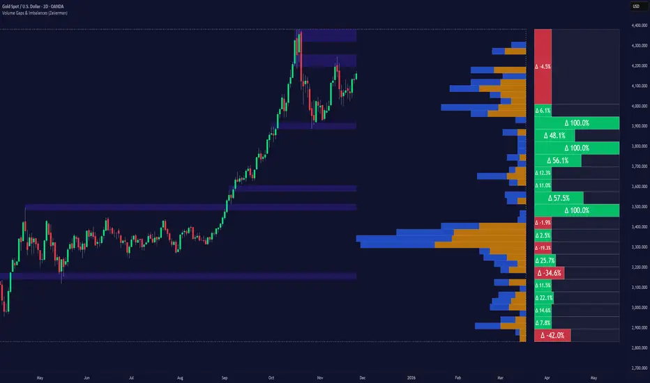
This shows the volume and volatility of each hour of the day for gold futures. As we can see, the most volume and volatility occur during the three hours around the RTH open at 8:00, 9:00, and 10:00 a.m.
Traders may want to isolate hours with the highest median volatility and volume to concentrate execution and avoid low-liquidity periods.
🔹 Assets Comparison
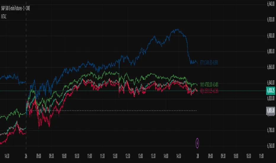
This tool allows us to compare different assets over the same period. In this case, we are comparing the hours of the day for 10-year notes, the S&P 500, silver, and the yen. Each asset has a different volatility profile throughout the day.
With the Delta feature enabled, we can clearly see the differences. The 10Y Notes move from 7:00 to 9:00 and from 2:00 to 9:00. The Yen moves from 7:00 to 9:00 and from 2:00 to 9:00. Silver moves from 8:00 to 10:00. The S&P 500 moves from 8:00 to 9:00 and from 14:00 to 15:00. All times are in exchange time.
🔹 Sizing & Coloring Graphs
Traders can adjust the width and height of the graphs, as well as the text size, at will.
Traders can choose from four different color configurations in the settings panel.
🔶 SETTINGS
Data: Select the type of data to display: Volume or Volatility.
Period: Select the time period to display: Month, Day of Month, Day of Week, or Hours.
Display delta between medians. Display the difference between the medians as a percentage. The smaller median is 0 and the larger median is 100. Enabling this feature highlights the differences between values.
🔹 Graph
Graph: Select the graph location.
Size: Select the graph size.
Width: Select the graph width.
Height: Select the height of the graph.
🔹 Style
Colors: Select a color map: Viridis, Plasma, Magma, or Custom.
Custom Cold: Select a custom color for cold (low values).
Custom Lukewarm: Select a custom color for lukewarm (medium values).
Custom Hot: Select a custom color for hot (high values).
אינדיקטור Pine Script®