Tims Smart Money COT-IndexThe **Tims Smart Money COT Index** analyzes the positions of different groups of market participants from the COT report (Commercials, Large Specs, Small Specs). It calculates their net positions and scales them relative to extremes of the last 24 weeks. It indicates bullish and bearish zones to identify market sentiments.
- Commercials (Smart Money)**: Often act against the trend, bullish from 80+.
- Large Specs (Retail Money)**: Trend-following, bullish from 80+.
- Small Specs**: Mostly impulsive, bullish from 80+.
The indicator helps to identify turning points in the market based on the behavior of the players.
חפש סקריפטים עבור "TIM投资动向"

[blackcat] L1 Tim Tillson IE/2Level: 1
Background
Before this script, I cannot find a IE/2 moving average script in tradingview. Although it is not so complex, it is meaningful to be the 1st Tim Tilson IE/2 script in tradingview community. IE/2 moving average was disclosed in "Smoothin Techniques For More Accurate Signals", Tim Tilson, S&C Magazine, Traders Tips, 01/1998.
Function
IE/2 is one of pre-studies created while T3 famous average was developing. It is calculated as (ILRS(n)+EPMA(n))/2. ILRS, is an integral of linear regression slope. In this moving average, the slope of a linear regression line is simply integrated as it is fitted in a moving window of length n across the data. The derivative of ILRS is the linear regression slope.EPMA is an end point moving average - it is the endpoint of the linear regression line of length n as it is fitted across the data. EPMA hugs the data more closely than a simple or exponential moving average of the same length.
The most popular method of interpreting a moving average is to compare the relationship between a moving average of the security's price with the security's price itself (or between several moving averages).
Inputs
Price --> price data to use
Period --> number of bars to use in calculation
Key Signal
Price --> Price Input.
IE/2 --> IE/2 Ouput.
Remarks
This is a Level 1 free and open source indicator.
Feedbacks are appreciated.

[blackcat] L1 Tim Tillson T3Level: 1
Background
T3 Moving Average is the responsive form of traditional moving averages. Presented in 1998 by Tim Tillson, T3 is also known as the Tillson Moving Averages. The thought behind the development of this technical indicator was to improve lag and false signals, which can be present in moving averages.
Function
The T3 indicator performs better than the ordinary moving averages. The reason for this is T3 Moving Average is built with the EMA (exponential moving average).
Its calculation is based on the sum of single EMA, double EMA, Triple EMA, and so on.
This gives the following equation:
T3 = c1*e6 + c2*e5 + c3*e4 + c4*e3…
Where
e3 = EMA (e2, Period)
e4 = EMA (e3, Period)
e5 = EMA (e4, Period)
e6 = EMA (e5, Period)
a is the volume factor, with a default value of 0.7 but you can also use 0.618
c1 = a^3
c2 = 3*a^2 + 3*a^3
c3 =6*a^2 – 3*a – 3*a^3
c4 = 1 + 3*a + a^3 + 3*a^2
When a trend appears, the price action stays above or below the trend line and doesn’t get disturbed from the price swing. The moving of the T3 and the lack of reversals can indicate the end of the trend. The T3 Moving Average produces signals just like moving averages, and similar trading conditions can be applied. If the price is above the T3 Moving Average and the indicator moves upward, this is a sign of a bullish trend. Here we may look to enter long. Conversely, if the price action is below the T3 Moving Average and the indicator moves downwards, a bearish trend appears. Here we may want to look for a short entry.
Key Signal
Price --> Price Input.
T3 --> T3 Ouput.
Remarks
This is a Level 1 free and open source indicator.
Feedbacks are appreciated.

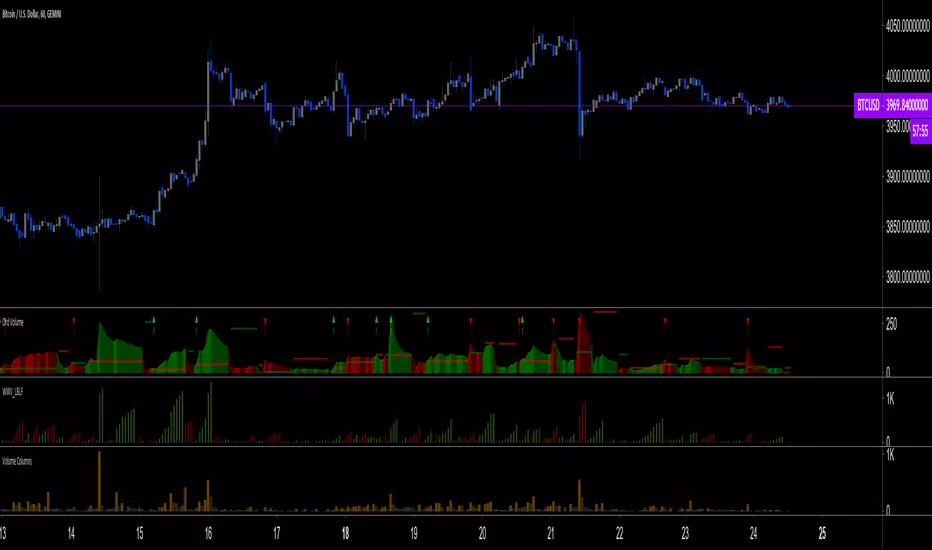
Ord Volume [LucF]Tim Ord came up with the Ord Volume concept. The idea is similar to Weis Wave , except that where Weis Wave keeps a cumulative tab of each wave’s successive volume columns, Ord Volume tracks the wave's average volume .
Features
You can choose to distinguish the area’s colors when the average is rising/falling (default).
You can show an EMA of the wave averages, which is different than an EMA on raw volume.
You can show (default) the last wave’s ending average over the current wave, to help in comparing relative levels.
You can change the length of the trend that needs to be broken for a new wave to start, as well as the price used in trend detection.
Use Cases
As with Weis Wave, what I look at first are three characteristics of the waves: their length, height and slope. I then compare those to the corresponding price movements, looking for discrepancies. For example, consecutive bearish waves of equal strength associated with lesser and lesser price movements are often a good indication of an impeding reversal.
Because Ord Volume uses average rather than cumulative volume, I find it is often easier to distinguish what is going on during waves, especially exhaustion at the end of waves.
Tim Ord has a method for entries and exits where he uses Ord Volume in conjunction with tests of support and resistance levels. Here are two articles published in 2004 where Ord explains his technique:
pr.b5z.net
n.b5z.net
Note
Being dependent on volume information as it is currently available in Pine, which does not include a practical way to retrieve delta volume information, the indicator suffers the same lack of precision as most other Pine-built volume indicators. For those not aware of the issue, the problem is that there is no way to distinguish the buying and selling volume (delta volume) in a bar, other than by looping through inside intervals using the security() function, which for me makes performance unsustainable in day to day use, while only providing an approximation of delta volume.

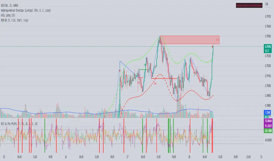
RSI Phi PhiSống để cho đi.
Phương pháp của sư phụ
Sống trong đời sống cần có một tấm lòng
Để làm gì, em biết không?
Để gió cuốn đi
Để gió cuốn đi
Gió cuốn đi cho mây qua dòng sông
Ngày vừa lên hay đêm xuống mênh mông
Ôi trái tim đang bay theo thời gian
Làm chiếc bóng đi rao lời dối gian
Những khi chiều tới, cần có một tiếng cười
Để ngậm ngùi theo lá bay
Rồi nước cuốn trôi
Rồi nước cuốn trôi
Hãy nghiêng đời xuống, nhìn suốt một mối tình
Chỉ lặng nhìn không nói năng
Để buốt trái tim
Để buốt trái tim
Trong trái tim con chim đau nằm yên
Ngủ dài lâu mang theo vết thương sâu
Một sớm mai, chim bay đi triền miên
Và tiếng hót tan trong trời gió lên
Hãy yêu ngày tới dù quá mệt kiếp người
Còn cuộc đời, ta cứ vui
Dù vắng bóng ai
Dù vắng bóng ai
Dù vắng bóng ai
Dù vắng bóng ai
Dù vắng bóng ai
RSI-Adaptive T3 [ChartPrime]The RSI-Adaptive T3 is a precision trend-following tool built around the legendary T3 smoothing algorithm developed by Tim Tillson , designed to enhance responsiveness while reducing lag compared to traditional moving averages. Current implementation takes it a step further by dynamically adapting the smoothing length based on real-time RSI conditions — allowing the T3 to “breathe” with market volatility. This dynamic length makes the curve faster in trending moves and smoother during consolidations.
To help traders visualize volatility and directional momentum, adaptive volatility bands are plotted around the T3 line, with visual crossover markers and a dynamic info panel on the chart. It’s ideal for identifying trend shifts, spotting momentum surges, and adapting strategy execution to the pace of the market.
HOIW IT WORKS
At its core, this indicator fuses two ideas:
The T3 Moving Average — a 6-stage recursively smoothed exponential average created by Tim Tillson , designed to reduce lag without sacrificing smoothness. It uses a volume factor to control curvature.
A Dynamic Length Engine — powered by the RSI. When RSI is low (market oversold), the T3 becomes shorter and more reactive. When RSI is high (overbought), the T3 becomes longer and smoother. This creates a feedback loop between price momentum and trend sensitivity.
// Step 1: Adaptive length via RSI
rsi = ta.rsi(src, rsiLen)
rsi_scale = 1 - rsi / 100
len = math.round(minLen + (maxLen - minLen) * rsi_scale)
pine_ema(src, length) =>
alpha = 2 / (length + 1)
sum = 0.0
sum := na(sum ) ? src : alpha * src + (1 - alpha) * nz(sum )
sum
// Step 2: T3 with adaptive length
e1 = pine_ema(src, len)
e2 = pine_ema(e1, len)
e3 = pine_ema(e2, len)
e4 = pine_ema(e3, len)
e5 = pine_ema(e4, len)
e6 = pine_ema(e5, len)
c1 = -v * v * v
c2 = 3 * v * v + 3 * v * v * v
c3 = -6 * v * v - 3 * v - 3 * v * v * v
c4 = 1 + 3 * v + v * v * v + 3 * v * v
t3 = c1 * e6 + c2 * e5 + c3 * e4 + c4 * e3
The result: an evolving trend line that adapts to market tempo in real-time.
KEY FEATURES
⯁ RSI-Based Adaptive Smoothing
The length of the T3 calculation dynamically adjusts between a Min Length and Max Length , based on the current RSI.
When RSI is low → the T3 shortens, tracking reversals faster.
When RSI is high → the T3 stretches, filtering out noise during euphoria phases.
Displayed length is shown in a floating table, colored on a gradient between min/max values.
⯁ T3 Calculation (Tim Tillson Method)
The script uses a 6-stage EMA cascade with a customizable Volume Factor (v) , as designed by Tillson (1998) .
Formula:
T3 = c1 * e6 + c2 * e5 + c3 * e4 + c4 * e3
This technique gives smoother yet faster curves than EMAs or DEMA/Triple EMA.
⯁ Visual Trend Direction & Transitions
The T3 line changes color dynamically:
Color Up (default: blue) → bullish curvature
Color Down (default: orange) → bearish curvature
Plot fill between T3 and delayed T3 creates a gradient ribbon to show momentum expansion/contraction.
Directional shift markers (“🞛”) are plotted when T3 crosses its own delayed value — helping traders spot trend flips or pullback entries.
⯁ Adaptive Volatility Bands
Optional upper/lower bands are plotted around the T3 line using a user-defined volatility window (default: 100).
Bands widen when volatility rises, and contract during compression — similar to Bollinger logic but centered on the adaptive T3.
Shaded band zones help frame breakout setups or mean-reversion zones.
⯁ Dynamic Info Table
A live stats panel shows:
Current adaptive length
Maximum smoothing (▲ MaxLen)
Minimum smoothing (▼ MinLen)
All values update in real time and are color-coded to match trend direction.
HOW TO USE
Use T3 crossovers to detect trend transitions, especially during periods of volatility compression.
Watch for volatility contraction in the bands — breakouts from narrow band periods often precede trend bursts.
The adaptive smoothing length can also be used to assess current market tempo — tighter = faster; wider = slower.
CONCLUSION
RSI-Adaptive T3 modernizes one of the most elegant smoothing algorithms in technical analysis with intelligent RSI responsiveness and built-in volatility bands. It gives traders a cleaner read on trend health, directional shifts, and expansion dynamics — all in a visually efficient package. Perfect for scalpers, swing traders, and algorithmic modelers alike, it delivers advanced logic in a plug-and-play format.

Six T3 Bands – Set to Any Time Frame [1000X]Script Description: Six T3 Bands – Set to Any Time Frame
This script leverages T3 lines, an advanced form of moving averages, to provide more adaptive and responsive indicators compared to traditional Moving Averages (MA) or Exponential Moving Averages (EMA). The T3 indicator, originally conceptualized by Tim Tillson in 1998, is known for its smoothness and reduced lag, making it a powerful tool for traders seeking precise market signals.
Features:
1 Adjustable Parameters:
◦ The script allows for the customization of six different T3 lines, each with adjustable lengths and "b values" (smoothing coefficients). This flexibility lets users fine-tune the indicators to fit various trading styles and market conditions.
◦ Users can set the reference timeframe for the T3 lines using the request.security function, enabling analysis across different timeframes. By default, the timeframe is set to the daily chart.
2 Calculation Method:
◦ The T3 lines are calculated using a multi-stage Exponential Moving Average (EMA) process. Specifically, the price data is smoothed through six stages of EMA calculations, with coefficients applied to produce the final T3 value. This method ensures the T3 lines are smoother and less laggy than traditional moving averages.
3 Usage:
◦ The T3 lines can be utilized to identify natural support and resistance levels within the market. By observing how the price interacts with these lines, traders can gain insights into potential reversal points or continuation patterns.
◦ The script's default settings are optimized for identifying these levels, but users are encouraged to adjust the parameters to match their specific trading strategies.
How to Use:
1 Customization:
◦ Access the script's settings to adjust the T3 lengths and "b values" for each of the six lines. This customization allows you to tailor the indicator to your preferred sensitivity and responsiveness.
◦ Set the reference timeframe according to your analysis needs. Whether you prefer intraday, daily, or longer-term charts, the T3 lines will remain set to the reference timeframe that you choose, while you focus your attention on the time frame of your choice.
2 Trading Strategies:
◦ Support and Resistance Trading: Use the T3 lines to identify key support and resistance zones. Look for price reactions around these lines to make informed trading decisions.
◦ Trend Confirmation: Combine the T3 lines with other technical indicators to confirm trends and filter out noise. The smoothness of the T3 lines helps in recognizing genuine trend changes.
Conclusion: This script builds on the foundational work of Tim Tillson and the classic T3 Average script by @HPotter (2014). Significant enhancements include making the "b value" an adjustable input and utilizing the request.security function to apply T3 lines to a specified timeframe. These improvements provide traders with greater control and adaptability, enhancing the practical utility of the T3 indicator.
The "Six T3 Bands – Set to Any Time Frame " script offers a useful tool for traders looking to enhance their technical analysis, both to visualize trend direction and to identify likely support and resistance levels. Its adaptive nature and customizable features make it a valuable addition to many trading strategies..

1000X Dual T3 Set to Any Time Frame1000X Dual T3 Set to Any Time Frame
The "1000X Dual T3 Set to Any Time Frame" is an enhancement of the well-known T3 indicator, building upon the T3 Average script by HPotter , which was itself based on Tim Wilson's work on smoothing techniques. This version provides two T3 lines, which is useful when adapting one each to the long and short trends on the same chart, with the added flexibility of setting the indicator to a higher time frame than the one you are currently trading. We also make the "b" value adjustable, creating a more sensitivity, adaptable indicator. This indicator is recommended as a trend filter or confirmation indicator in trading strategies.
Key Features
Dual Trend Analysis: The dual T3 offers a view of long and short trends to aid in better optimized market analysis. This avoids the problem with using a single T3 line to filter tradable price action for both long and short sides, which forces one to compromise performance in order to achieve profitability in both directions.
Timeframe Customization: This indicator can be set to a desired timeframe while trading another. For example, the T3 can be set as a trend filter on the daily or weekly time frame to separate bull and bear markets, even as you work with other indicators on a chart set to a lower time frame. Set the time frame in the inputs, using minutes (15, 60, 240, etc.) or using D, W, and M.
Preserved T3 Script: Like the powerful HPotter script on which it builds, this indicator leverages EMA-based T3 smoothing calculations for smooth and responsive trend lines.
B Value adjustability: Given the role of the b value in smoothing and sensitivity, I have found it beneficial to make the b value an adjustable input as well. A higher b value will make the T3 line more responsive to recent price changes, making it closer to the actual price movements but potentially more susceptible to market noise.
Visual Trend Indicators: In addition to filtering markets using the "above or below" approach, this script provides colour coding to delineate trend directions.
Acknowledgments
As stated, this work is a tribute to the foundational contributions of Tim Wilson and the subsequent development by HPotter whose script was the basis of this one. The enhancements in this version aim to provide added value to the trading community.

Adaptive Fisherized Z-scoreHello Fellas,
It's time for a new adaptive fisherized indicator of me, where I apply adaptive length and more on a classic indicator.
Today, I chose the Z-score, also called standard score, as indicator of interest.
Special Features
Advanced Smoothing: JMA, T3, Hann Window and Super Smoother
Adaptive Length Algorithms: In-Phase Quadrature, Homodyne Discriminator, Median and Hilbert Transform
Inverse Fisher Transform (IFT)
Signals: Enter Long, Enter Short, Exit Long and Exit Short
Bar Coloring: Presents the trade state as bar colors
Band Levels: Changes the band levels
Decision Making
When you create such a mod you need to think about which concepts are the best to conclude. I decided to take Inverse Fisher Transform instead of normalization to make a version which fits to a fixed scale to avoid the usual distortion created by normalization.
Moreover, I chose JMA, T3, Hann Window and Super Smoother, because JMA and T3 are the bleeding-edge MA's at the moment with the best balance of lag and responsiveness. Additionally, I chose Hann Window and Super Smoother because of their extraordinary smoothing capabilities and because Ehlers favours them.
Furthermore, I decided to choose the half length of the dominant cycle instead of the full dominant cycle to make the indicator more responsive which is very important for a signal emitter like Z-score. Signal emitters always need to be faster or have the same speed as the filters they are combined with.
Usage
The Z-score is a low timeframe scalper which works best during choppy/ranging phases. The direction you should trade is determined by the last trend change. E.g. when the last trend change was from bearish market to bullish market and you are now in a choppy/ranging phase confirmed by e.g. Chop Zone or KAMA slope you want to do long trades.
Interpretation
The Z-score indicator is a momentum indicator which shows the number of standard deviations by which the value of a raw score (price/source) is above or below the mean value of what is being observed or measured. Easily explained, it is almost the same as Bollinger Bands with another visual representation form.
Signals
B -> Buy -> Z-score crosses above lower band
S -> Short -> Z-score crosses below upper band
BE -> Buy Exit -> Z-score crosses above 0
SE -> Sell Exit -> Z-score crosses below 0
If you were reading till here, thank you already. Now, follows a bunch of knowledge for people who don't know the concepts I talk about.
T3
The T3 moving average, short for "Tim Tillson's Triple Exponential Moving Average," is a technical indicator used in financial markets and technical analysis to smooth out price data over a specific period. It was developed by Tim Tillson, a software project manager at Hewlett-Packard, with expertise in Mathematics and Computer Science.
The T3 moving average is an enhancement of the traditional Exponential Moving Average (EMA) and aims to overcome some of its limitations. The primary goal of the T3 moving average is to provide a smoother representation of price trends while minimizing lag compared to other moving averages like Simple Moving Average (SMA), Weighted Moving Average (WMA), or EMA.
To compute the T3 moving average, it involves a triple smoothing process using exponential moving averages. Here's how it works:
Calculate the first exponential moving average (EMA1) of the price data over a specific period 'n.'
Calculate the second exponential moving average (EMA2) of EMA1 using the same period 'n.'
Calculate the third exponential moving average (EMA3) of EMA2 using the same period 'n.'
The formula for the T3 moving average is as follows:
T3 = 3 * (EMA1) - 3 * (EMA2) + (EMA3)
By applying this triple smoothing process, the T3 moving average is intended to offer reduced noise and improved responsiveness to price trends. It achieves this by incorporating multiple time frames of the exponential moving averages, resulting in a more accurate representation of the underlying price action.
JMA
The Jurik Moving Average (JMA) is a technical indicator used in trading to predict price direction. Developed by Mark Jurik, it’s a type of weighted moving average that gives more weight to recent market data rather than past historical data.
JMA is known for its superior noise elimination. It’s a causal, nonlinear, and adaptive filter, meaning it responds to changes in price action without introducing unnecessary lag. This makes JMA a world-class moving average that tracks and smooths price charts or any market-related time series with surprising agility.
In comparison to other moving averages, such as the Exponential Moving Average (EMA), JMA is known to track fast price movement more accurately. This allows traders to apply their strategies to a more accurate picture of price action.
Inverse Fisher Transform
The Inverse Fisher Transform is a transform used in DSP to alter the Probability Distribution Function (PDF) of a signal or in our case of indicators.
The result of using the Inverse Fisher Transform is that the output has a very high probability of being either +1 or –1. This bipolar probability distribution makes the Inverse Fisher Transform ideal for generating an indicator that provides clear buy and sell signals.
Hann Window
The Hann function (aka Hann Window) is named after the Austrian meteorologist Julius von Hann. It is a window function used to perform Hann smoothing.
Super Smoother
The Super Smoother uses a special mathematical process for the smoothing of data points.
The Super Smoother is a technical analysis indicator designed to be smoother and with less lag than a traditional moving average.
Adaptive Length
Length based on the dominant cycle length measured by a "dominant cycle measurement" algorithm.
Happy Trading!
Best regards,
simwai
---
Credits to
@cheatcountry
@everget
@loxx
@DasanC
@blackcat1402

Goertzel Adaptive JMA T3Hello Fellas,
The Goertzel Adaptive JMA T3 is a powerful indicator that combines my own created Goertzel adaptive length with Jurik and T3 Moving Averages. The primary intention of the indicator is to demonstrate the new adaptive length algorithm by applying it on bleeding-edge MAs.
It is useable like any moving average, and the new Goertzel adaptive length algorithm can be used to make own indicators Goertzel adaptive.
Used Adaptive Length Algorithms
Normalized Goertzel Power: This uses the normalized power of the Goertzel algorithm to compute an adaptive length without the special operations, like detrending, Ehlers uses for his DFT adaptive length.
Ehlers Mod: This uses the Goertzel algorithm instead of the DFT, originally used by Ehlers, to compute a modified version of his original approach, which sticks as close as possible to the original approach.
Scoring System
The scoring system determines if bars are red or green and collects them.
Then, it goes through all collected red and green bars and checks how big they are and if they are above or below the selected MA. It is positive when green bars are under MA or when red bars are above MA.
Then, it accumulates the size for all positive green bars and for all positive red bars. The same happens for negative green and red bars.
Finally, it calculates the score by ((positiveGreenBars + positiveRedBars) / (negativeGreenBars + negativeRedBars)) * 100 with the scale 0–100.
Signals
Is the price above MA? -> bullish market
Is the price below MA? -> bearish market
Usage
Adjust the settings to reach the highest score, and enjoy an outstanding adaptive MA.
It should be useable on all timeframes. It is recommended to use the indicator on the timeframe where you can get the highest score.
Now, follows a bunch of knowledge for people who don't know about the concepts used here.
T3
The T3 moving average, short for "Tim Tillson's Triple Exponential Moving Average," is a technical indicator used in financial markets and technical analysis to smooth out price data over a specific period. It was developed by Tim Tillson, a software project manager at Hewlett-Packard, with expertise in Mathematics and Computer Science.
The T3 moving average is an enhancement of the traditional Exponential Moving Average (EMA) and aims to overcome some of its limitations. The primary goal of the T3 moving average is to provide a smoother representation of price trends while minimizing lag compared to other moving averages like Simple Moving Average (SMA), Weighted Moving Average (WMA), or EMA.
To compute the T3 moving average, it involves a triple smoothing process using exponential moving averages. Here's how it works:
Calculate the first exponential moving average (EMA1) of the price data over a specific period 'n.'
Calculate the second exponential moving average (EMA2) of EMA1 using the same period 'n.'
Calculate the third exponential moving average (EMA3) of EMA2 using the same period 'n.'
The formula for the T3 moving average is as follows:
T3 = 3 * (EMA1) - 3 * (EMA2) + (EMA3)
By applying this triple smoothing process, the T3 moving average is intended to offer reduced noise and improved responsiveness to price trends. It achieves this by incorporating multiple time frames of the exponential moving averages, resulting in a more accurate representation of the underlying price action.
JMA
The Jurik Moving Average (JMA) is a technical indicator used in trading to predict price direction. Developed by Mark Jurik, it’s a type of weighted moving average that gives more weight to recent market data rather than past historical data.
JMA is known for its superior noise elimination. It’s a causal, nonlinear, and adaptive filter, meaning it responds to changes in price action without introducing unnecessary lag. This makes JMA a world-class moving average that tracks and smooths price charts or any market-related time series with surprising agility.
In comparison to other moving averages, such as the Exponential Moving Average (EMA), JMA is known to track fast price movement more accurately. This allows traders to apply their strategies to a more accurate picture of price action.
Goertzel Algorithm
The Goertzel algorithm is a technique in digital signal processing (DSP) for efficient evaluation of individual terms of the Discrete Fourier Transform (DFT). It's particularly useful when you need to compute a small number of selected frequency components. Unlike direct DFT calculations, the Goertzel algorithm applies a single real-valued coefficient at each iteration, using real-valued arithmetic for real-valued input sequences. This makes it more numerically efficient when computing a small number of selected frequency components¹.
Discrete Fourier Transform
The Discrete Fourier Transform (DFT) is a mathematical technique used in signal processing to convert a finite sequence of equally-spaced samples of a function into a same-length sequence of equally-spaced samples of the discrete-time Fourier transform (DTFT), which is a complex-valued function of frequency . The DFT provides a frequency domain representation of the original input sequence .
Usage of DFT/Goertzel In Adaptive Length Algorithms
Adaptive length algorithms are automated trading systems that can dynamically adjust their parameters in response to real-time market data. This adaptability enables them to optimize their trading strategies as market conditions fluctuate. Both the Goertzel algorithm and DFT can be used in these algorithms to analyze market data and detect cycles or patterns, which can then be used to adjust the parameters of the trading strategy.
The Goertzel algorithm is more efficient than the DFT when you need to compute a small number of selected frequency components. However, for covering a full spectrum, the Goertzel algorithm has a higher order of complexity than fast Fourier transform (FFT) algorithms.
I hope this can help you somehow.
Thanks for reading, and keep it up.
Best regards,
simwai
---
Credits to:
@ClassicScott
@yatrader2
@cheatcountry
@loxx

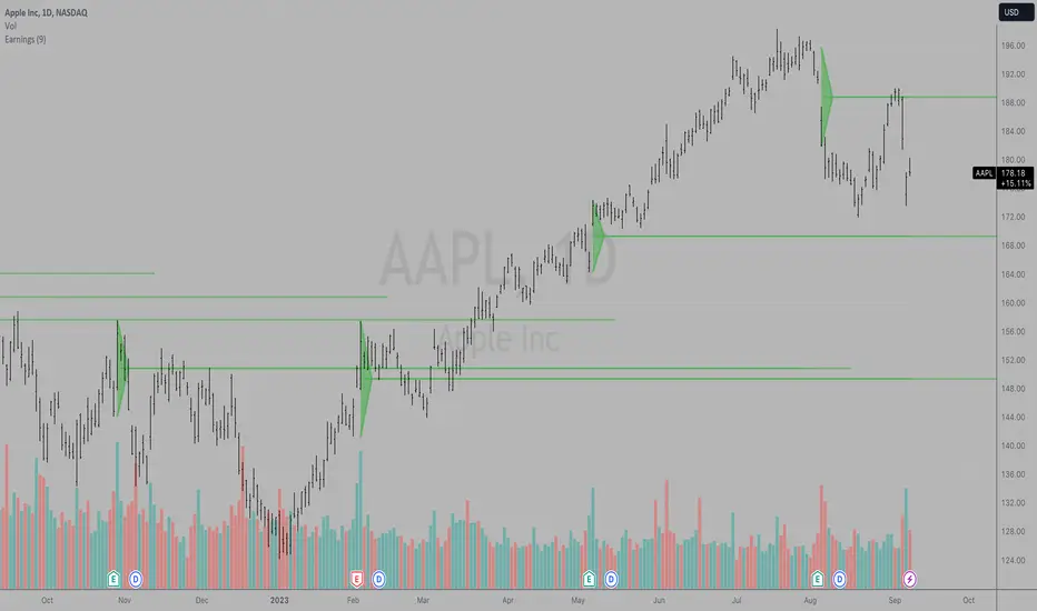
Earnings LevelsI am proud to announce that the formerly secret "Key Earnings Levels" graphing tool will be freely available to TradingView users whereas before it was only available by monthly or annual subscription since its invention here at TradingView many years ago by Tim West. TradingView code writers wrote the original code for using this powerful tool and then Johannes Falkenburg re-wrote the code several years ago.
The most important FOUR days a year in a stock chart are the days that the company gives its quarterly update. Since the GRAND majority of companies have earnings, the indicator is called the "Key Earnings Level", or KEL for short. The unique part of the release of the quarterly update is that it can be "before the open" or "after the close" and the price action leading up to the earnings and immediately after the earnings are useful for future reference, as you'll see shortly.
The Key Earnings indicator plots a triangle for the range around the day before and the day after earnings and draws a mid-point line to capture the over/under level for that report. That mid-point line is then extended into the future for a minimum of one quarter until the next earnings report and as long as a year with the current code.
This triangle plot allows you to see how a stock is trading RELATIVE TO where it was trading when earnings were announced and when a glimpse into the current quarter along with projections for the upcoming year.
Simply put: Key Earnings Levels are the easiest way to see how a stock is doing relative to the most important four days a year.
You can devise your own trading strategies around these levels, but I want you to have this information so you can see it and know it too. I've kept this little secret of Key Hidden Levels to myself and my followers in the Key Hidden Levels Chat Room here at TradingView for far too long. I have occasionally published charts with the Key Earnings Levels but have not made the code freely available to TradingView subscribers.
If anyone has paid me for access to these indicators and wants a refund, I will be glad to do that. This is too important to keep from everyone any longer. I think it is essential to make this available to everyone to make sure we all have the most advantage we can get when investing and trading in the markets.
I hope you can all find the powerful benefit from using Key Earnings Levels and please thank Johannes Falkenburg aka @Vollchaot here at TradingView for writing the latest version of this code.
The idea itself came from using TradingView and the powerful graphing and layout features here to track our observations and to do research. Thank you TradingView for such a great product.
I look forward to answering any questions.
Sincerely,
Tim West
EMA-Deviation-Corrected T3 [Loxx]EMA-Deviation-Corrected T3 is a T3 moving average that uses EMA deviation correcting to produce signals. This comes via the beloved genius Mladen.
The origin of the correcting algorithm can be attributed to Dr. Alexander Uhl, who developed a method to filter the moving average and identify signals. Originally, this method utilized standard deviation as a measure to correct the average values.
However, the current indicator in question employs a modified version of the correcting method. Instead of using standard deviation for calculation, it uses EMA deviation, which stands for Exponential Moving Average deviation. The idea behind using EMA deviation is two-fold:
Efficiency: EMA deviation can be calculated faster than standard deviation, resulting in more efficient code execution.
Signal Reduction: Surprisingly, this modified "correcting" approach generates fewer signals compared to using standard deviation. This is because EMA deviation is more responsive to price changes, making the correcting process less sensitive to whipsaws or false signals.
What is T3?
The T3 moving average, short for "Tim Tillson's Triple Exponential Moving Average," is a technical indicator used in financial markets and technical analysis to smooth out price data over a specific period. It was developed by Tim Tillson, a software project manager at Hewlett-Packard, with expertise in Mathematics and Computer Science.
The T3 moving average is an enhancement of the traditional Exponential Moving Average (EMA) and aims to overcome some of its limitations. The primary goal of the T3 moving average is to provide a smoother representation of price trends while minimizing lag compared to other moving averages like Simple Moving Average (SMA), Weighted Moving Average (WMA), or EMA.
To compute the T3 moving average, it involves a triple smoothing process using exponential moving averages. Here's how it works:
Calculate the first exponential moving average (EMA1) of the price data over a specific period 'n.'
Calculate the second exponential moving average (EMA2) of EMA1 using the same period 'n.'
Calculate the third exponential moving average (EMA3) of EMA2 using the same period 'n.'
The formula for the T3 moving average is as follows:
T3 = 3 * (EMA1) - 3 * (EMA2) + (EMA3)
By applying this triple smoothing process, the T3 moving average is intended to offer reduced noise and improved responsiveness to price trends. It achieves this by incorporating multiple time frames of the exponential moving averages, resulting in a more accurate representation of the underlying price action.
Included
Bar coloring
Signals
Alerts
Loxx's Expanded Source Types

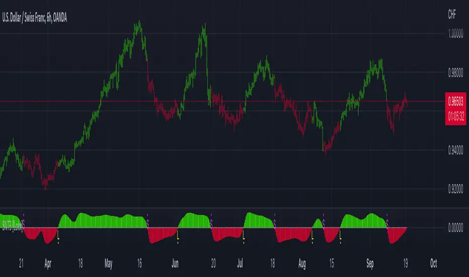
T3 OscillatorTL;DR - An Oscillator based on T3 moving average
The T3 moving average is a well known moving average created by Tim TIllson. Oscillator values are created by using the simple formula "source (close by default) - T3 moving average". Tim Tillson used a "volume factor" of 0.7 in his original T3 calculation. I changed this value to 0.618 and added the option to change it if needed/wanted. I also added alarms for zero line crossing upwards and downward, a smoothing option and custom time frames.
Compared to other oscillators like TSI, MACD etc. I observed better signals, especially in trending market situations, from the T3 oscillator (I tested Forex and Crypto).
Usage is simple: If the oscillator is above 0 it indicates a bearish trend. If below 0 it indicates a bullish trend. -> Really simple to use. However it can also be used to determine micro trends and reversals when combined with price action analysis. To keeps things simple I have not added a moving average like many other oscillators because I think it is confusing and does not help (in this particular case).
P.S. I haven't found a T3 oscillator on Trading View. Code is free - do whatever you want with it ;)

STD-Adaptive T3 [Loxx]STD-Adaptive T3 is a standard deviation adaptive T3 moving average filter. This indicator acts more like a trend overlay indicator with gradient coloring.
What is the T3 moving average?
Better Moving Averages Tim Tillson
November 1, 1998
Tim Tillson is a software project manager at Hewlett-Packard, with degrees in Mathematics and Computer Science. He has privately traded options and equities for 15 years.
Introduction
"Digital filtering includes the process of smoothing, predicting, differentiating, integrating, separation of signals, and removal of noise from a signal. Thus many people who do such things are actually using digital filters without realizing that they are; being unacquainted with the theory, they neither understand what they have done nor the possibilities of what they might have done."
This quote from R. W. Hamming applies to the vast majority of indicators in technical analysis . Moving averages, be they simple, weighted, or exponential, are lowpass filters; low frequency components in the signal pass through with little attenuation, while high frequencies are severely reduced.
"Oscillator" type indicators (such as MACD , Momentum, Relative Strength Index ) are another type of digital filter called a differentiator.
Tushar Chande has observed that many popular oscillators are highly correlated, which is sensible because they are trying to measure the rate of change of the underlying time series, i.e., are trying to be the first and second derivatives we all learned about in Calculus.
We use moving averages (lowpass filters) in technical analysis to remove the random noise from a time series, to discern the underlying trend or to determine prices at which we will take action. A perfect moving average would have two attributes:
It would be smooth, not sensitive to random noise in the underlying time series. Another way of saying this is that its derivative would not spuriously alternate between positive and negative values.
It would not lag behind the time series it is computed from. Lag, of course, produces late buy or sell signals that kill profits.
The only way one can compute a perfect moving average is to have knowledge of the future, and if we had that, we would buy one lottery ticket a week rather than trade!
Having said this, we can still improve on the conventional simple, weighted, or exponential moving averages. Here's how:
Two Interesting Moving Averages
We will examine two benchmark moving averages based on Linear Regression analysis.
In both cases, a Linear Regression line of length n is fitted to price data.
I call the first moving average ILRS, which stands for Integral of Linear Regression Slope. One simply integrates the slope of a linear regression line as it is successively fitted in a moving window of length n across the data, with the constant of integration being a simple moving average of the first n points. Put another way, the derivative of ILRS is the linear regression slope. Note that ILRS is not the same as a SMA ( simple moving average ) of length n, which is actually the midpoint of the linear regression line as it moves across the data.
We can measure the lag of moving averages with respect to a linear trend by computing how they behave when the input is a line with unit slope. Both SMA (n) and ILRS(n) have lag of n/2, but ILRS is much smoother than SMA .
Our second benchmark moving average is well known, called EPMA or End Point Moving Average. It is the endpoint of the linear regression line of length n as it is fitted across the data. EPMA hugs the data more closely than a simple or exponential moving average of the same length. The price we pay for this is that it is much noisier (less smooth) than ILRS, and it also has the annoying property that it overshoots the data when linear trends are present.
However, EPMA has a lag of 0 with respect to linear input! This makes sense because a linear regression line will fit linear input perfectly, and the endpoint of the LR line will be on the input line.
These two moving averages frame the tradeoffs that we are facing. On one extreme we have ILRS, which is very smooth and has considerable phase lag. EPMA has 0 phase lag, but is too noisy and overshoots. We would like to construct a better moving average which is as smooth as ILRS, but runs closer to where EPMA lies, without the overshoot.
A easy way to attempt this is to split the difference, i.e. use (ILRS(n)+EPMA(n))/2. This will give us a moving average (call it IE /2) which runs in between the two, has phase lag of n/4 but still inherits considerable noise from EPMA. IE /2 is inspirational, however. Can we build something that is comparable, but smoother? Figure 1 shows ILRS, EPMA, and IE /2.
Filter Techniques
Any thoughtful student of filter theory (or resolute experimenter) will have noticed that you can improve the smoothness of a filter by running it through itself multiple times, at the cost of increasing phase lag.
There is a complementary technique (called twicing by J.W. Tukey) which can be used to improve phase lag. If L stands for the operation of running data through a low pass filter, then twicing can be described by:
L' = L(time series) + L(time series - L(time series))
That is, we add a moving average of the difference between the input and the moving average to the moving average. This is algebraically equivalent to:
2L-L(L)
This is the Double Exponential Moving Average or DEMA , popularized by Patrick Mulloy in TASAC (January/February 1994).
In our taxonomy, DEMA has some phase lag (although it exponentially approaches 0) and is somewhat noisy, comparable to IE /2 indicator.
We will use these two techniques to construct our better moving average, after we explore the first one a little more closely.
Fixing Overshoot
An n-day EMA has smoothing constant alpha=2/(n+1) and a lag of (n-1)/2.
Thus EMA (3) has lag 1, and EMA (11) has lag 5. Figure 2 shows that, if I am willing to incur 5 days of lag, I get a smoother moving average if I run EMA (3) through itself 5 times than if I just take EMA (11) once.
This suggests that if EPMA and DEMA have 0 or low lag, why not run fast versions (eg DEMA (3)) through themselves many times to achieve a smooth result? The problem is that multiple runs though these filters increase their tendency to overshoot the data, giving an unusable result. This is because the amplitude response of DEMA and EPMA is greater than 1 at certain frequencies, giving a gain of much greater than 1 at these frequencies when run though themselves multiple times. Figure 3 shows DEMA (7) and EPMA(7) run through themselves 3 times. DEMA^3 has serious overshoot, and EPMA^3 is terrible.
The solution to the overshoot problem is to recall what we are doing with twicing:
DEMA (n) = EMA (n) + EMA (time series - EMA (n))
The second term is adding, in effect, a smooth version of the derivative to the EMA to achieve DEMA . The derivative term determines how hot the moving average's response to linear trends will be. We need to simply turn down the volume to achieve our basic building block:
EMA (n) + EMA (time series - EMA (n))*.7;
This is algebraically the same as:
EMA (n)*1.7-EMA( EMA (n))*.7;
I have chosen .7 as my volume factor, but the general formula (which I call "Generalized Dema") is:
GD (n,v) = EMA (n)*(1+v)-EMA( EMA (n))*v,
Where v ranges between 0 and 1. When v=0, GD is just an EMA , and when v=1, GD is DEMA . In between, GD is a cooler DEMA . By using a value for v less than 1 (I like .7), we cure the multiple DEMA overshoot problem, at the cost of accepting some additional phase delay. Now we can run GD through itself multiple times to define a new, smoother moving average T3 that does not overshoot the data:
T3(n) = GD ( GD ( GD (n)))
In filter theory parlance, T3 is a six-pole non-linear Kalman filter. Kalman filters are ones which use the error (in this case (time series - EMA (n)) to correct themselves. In Technical Analysis , these are called Adaptive Moving Averages; they track the time series more aggressively when it is making large moves.
Included
Bar coloring
Loxx's Expanded Source Types

Softmax Normalized T3 Histogram [Loxx]Softmax Normalized T3 Histogram is a T3 moving average that is morphed into a normalized oscillator from -1 to 1.
What is the Softmax function?
The softmax function, also known as softargmax: or normalized exponential function, converts a vector of K real numbers into a probability distribution of K possible outcomes. It is a generalization of the logistic function to multiple dimensions, and used in multinomial logistic regression. The softmax function is often used as the last activation function of a neural network to normalize the output of a network to a probability distribution over predicted output classes, based on Luce's choice axiom.
What is the T3 moving average?
Better Moving Averages Tim Tillson
November 1, 1998
Tim Tillson is a software project manager at Hewlett-Packard, with degrees in Mathematics and Computer Science. He has privately traded options and equities for 15 years.
Introduction
"Digital filtering includes the process of smoothing, predicting, differentiating, integrating, separation of signals, and removal of noise from a signal. Thus many people who do such things are actually using digital filters without realizing that they are; being unacquainted with the theory, they neither understand what they have done nor the possibilities of what they might have done."
This quote from R. W. Hamming applies to the vast majority of indicators in technical analysis . Moving averages, be they simple, weighted, or exponential, are lowpass filters; low frequency components in the signal pass through with little attenuation, while high frequencies are severely reduced.
"Oscillator" type indicators (such as MACD , Momentum, Relative Strength Index ) are another type of digital filter called a differentiator.
Tushar Chande has observed that many popular oscillators are highly correlated, which is sensible because they are trying to measure the rate of change of the underlying time series, i.e., are trying to be the first and second derivatives we all learned about in Calculus.
We use moving averages (lowpass filters) in technical analysis to remove the random noise from a time series, to discern the underlying trend or to determine prices at which we will take action. A perfect moving average would have two attributes:
It would be smooth, not sensitive to random noise in the underlying time series. Another way of saying this is that its derivative would not spuriously alternate between positive and negative values.
It would not lag behind the time series it is computed from. Lag, of course, produces late buy or sell signals that kill profits.
The only way one can compute a perfect moving average is to have knowledge of the future, and if we had that, we would buy one lottery ticket a week rather than trade!
Having said this, we can still improve on the conventional simple, weighted, or exponential moving averages. Here's how:
Two Interesting Moving Averages
We will examine two benchmark moving averages based on Linear Regression analysis.
In both cases, a Linear Regression line of length n is fitted to price data.
I call the first moving average ILRS, which stands for Integral of Linear Regression Slope. One simply integrates the slope of a linear regression line as it is successively fitted in a moving window of length n across the data, with the constant of integration being a simple moving average of the first n points. Put another way, the derivative of ILRS is the linear regression slope. Note that ILRS is not the same as a SMA ( simple moving average ) of length n, which is actually the midpoint of the linear regression line as it moves across the data.
We can measure the lag of moving averages with respect to a linear trend by computing how they behave when the input is a line with unit slope. Both SMA (n) and ILRS(n) have lag of n/2, but ILRS is much smoother than SMA .
Our second benchmark moving average is well known, called EPMA or End Point Moving Average. It is the endpoint of the linear regression line of length n as it is fitted across the data. EPMA hugs the data more closely than a simple or exponential moving average of the same length. The price we pay for this is that it is much noisier (less smooth) than ILRS, and it also has the annoying property that it overshoots the data when linear trends are present.
However, EPMA has a lag of 0 with respect to linear input! This makes sense because a linear regression line will fit linear input perfectly, and the endpoint of the LR line will be on the input line.
These two moving averages frame the tradeoffs that we are facing. On one extreme we have ILRS, which is very smooth and has considerable phase lag. EPMA has 0 phase lag, but is too noisy and overshoots. We would like to construct a better moving average which is as smooth as ILRS, but runs closer to where EPMA lies, without the overshoot.
A easy way to attempt this is to split the difference, i.e. use (ILRS(n)+EPMA(n))/2. This will give us a moving average (call it IE /2) which runs in between the two, has phase lag of n/4 but still inherits considerable noise from EPMA. IE /2 is inspirational, however. Can we build something that is comparable, but smoother? Figure 1 shows ILRS, EPMA, and IE /2.
Filter Techniques
Any thoughtful student of filter theory (or resolute experimenter) will have noticed that you can improve the smoothness of a filter by running it through itself multiple times, at the cost of increasing phase lag.
There is a complementary technique (called twicing by J.W. Tukey) which can be used to improve phase lag. If L stands for the operation of running data through a low pass filter, then twicing can be described by:
L' = L(time series) + L(time series - L(time series))
That is, we add a moving average of the difference between the input and the moving average to the moving average. This is algebraically equivalent to:
2L-L(L)
This is the Double Exponential Moving Average or DEMA , popularized by Patrick Mulloy in TASAC (January/February 1994).
In our taxonomy, DEMA has some phase lag (although it exponentially approaches 0) and is somewhat noisy, comparable to IE /2 indicator.
We will use these two techniques to construct our better moving average, after we explore the first one a little more closely.
Fixing Overshoot
An n-day EMA has smoothing constant alpha=2/(n+1) and a lag of (n-1)/2.
Thus EMA (3) has lag 1, and EMA (11) has lag 5. Figure 2 shows that, if I am willing to incur 5 days of lag, I get a smoother moving average if I run EMA (3) through itself 5 times than if I just take EMA (11) once.
This suggests that if EPMA and DEMA have 0 or low lag, why not run fast versions (eg DEMA (3)) through themselves many times to achieve a smooth result? The problem is that multiple runs though these filters increase their tendency to overshoot the data, giving an unusable result. This is because the amplitude response of DEMA and EPMA is greater than 1 at certain frequencies, giving a gain of much greater than 1 at these frequencies when run though themselves multiple times. Figure 3 shows DEMA (7) and EPMA(7) run through themselves 3 times. DEMA^3 has serious overshoot, and EPMA^3 is terrible.
The solution to the overshoot problem is to recall what we are doing with twicing:
DEMA (n) = EMA (n) + EMA (time series - EMA (n))
The second term is adding, in effect, a smooth version of the derivative to the EMA to achieve DEMA . The derivative term determines how hot the moving average's response to linear trends will be. We need to simply turn down the volume to achieve our basic building block:
EMA (n) + EMA (time series - EMA (n))*.7;
This is algebraically the same as:
EMA (n)*1.7-EMA( EMA (n))*.7;
I have chosen .7 as my volume factor, but the general formula (which I call "Generalized Dema") is:
GD (n,v) = EMA (n)*(1+v)-EMA( EMA (n))*v,
Where v ranges between 0 and 1. When v=0, GD is just an EMA , and when v=1, GD is DEMA . In between, GD is a cooler DEMA . By using a value for v less than 1 (I like .7), we cure the multiple DEMA overshoot problem, at the cost of accepting some additional phase delay. Now we can run GD through itself multiple times to define a new, smoother moving average T3 that does not overshoot the data:
T3(n) = GD ( GD ( GD (n)))
In filter theory parlance, T3 is a six-pole non-linear Kalman filter. Kalman filters are ones which use the error (in this case (time series - EMA (n)) to correct themselves. In Technical Analysis , these are called Adaptive Moving Averages; they track the time series more aggressively when it is making large moves.
Included:
Bar coloring
Signals
Alerts
Loxx's Expanded Source Types
Step Generalized Double DEMA (ATR based) [Loxx]Step Generalized Double DEMA (ATR based) works like a T3 moving average but is less smooth. This is on purpose to catch more signals. The addition of ATR stepped filtering reduces noise while maintaining signal integrity. This one comes via Mr. Tools.
Theory:
The double exponential moving average (DEMA), was developed by Patrick Mulloy in an attempt to reduce the amount of lag time found in traditional moving averages. It was first introduced in the February 1994 issue of the magazine Technical Analysis of Stocks & Commodities in Mulloy's article "Smoothing Data with Faster Moving Averages". The way to calculate is the following :
The Double Exponential Moving Average calculations are based combinations of a single EMA and double EMA into a new EMA:
1. Calculate EMA
2. Calculate Smoothed EMA by applying EMA with the same period to the EMA calculated in the first step
3. Calculate DEMA
DEMA = (2 * EMA) - (Smoothed EMA)
This version:
For our purposes here, we are using Tim Tillson's (the inventor of T3) work, specifically, we are using the GDEMA of GDEMA for calculation (which is the "middle step" of T3 calculation). Since there are no versions showing that "middle step, this version covers that too. The result is smoother than Generalized DEMA, but is less smooth than T3 - one has to do some experimenting in order to find the optimal way to use it, but in any case, since it is "faster" than the T3 (Tim Tillson T3) and still smooth, it looks like a good compromise between speed and smoothness.
Usage:
You can use it as any regular average or you can use the color change of the indicator as a signal.
Included
Alerts
Signals
Bar coloring
Loxx's Expanded Source Types
T3 Velocity Candles [Loxx]T3 Velocity Candles is a candle coloring overlay that calculates its gradient coloring using T3 velocity.
What is the T3 moving average?
Better Moving Averages Tim Tillson
November 1, 1998
Tim Tillson is a software project manager at Hewlett-Packard, with degrees in Mathematics and Computer Science. He has privately traded options and equities for 15 years.
Introduction
"Digital filtering includes the process of smoothing, predicting, differentiating, integrating, separation of signals, and removal of noise from a signal. Thus many people who do such things are actually using digital filters without realizing that they are; being unacquainted with the theory, they neither understand what they have done nor the possibilities of what they might have done."
This quote from R. W. Hamming applies to the vast majority of indicators in technical analysis . Moving averages, be they simple, weighted, or exponential, are lowpass filters; low frequency components in the signal pass through with little attenuation, while high frequencies are severely reduced.
"Oscillator" type indicators (such as MACD , Momentum, Relative Strength Index ) are another type of digital filter called a differentiator.
Tushar Chande has observed that many popular oscillators are highly correlated, which is sensible because they are trying to measure the rate of change of the underlying time series, i.e., are trying to be the first and second derivatives we all learned about in Calculus.
We use moving averages (lowpass filters) in technical analysis to remove the random noise from a time series, to discern the underlying trend or to determine prices at which we will take action. A perfect moving average would have two attributes:
It would be smooth, not sensitive to random noise in the underlying time series. Another way of saying this is that its derivative would not spuriously alternate between positive and negative values.
It would not lag behind the time series it is computed from. Lag, of course, produces late buy or sell signals that kill profits.
The only way one can compute a perfect moving average is to have knowledge of the future, and if we had that, we would buy one lottery ticket a week rather than trade!
Having said this, we can still improve on the conventional simple, weighted, or exponential moving averages. Here's how:
Two Interesting Moving Averages
We will examine two benchmark moving averages based on Linear Regression analysis.
In both cases, a Linear Regression line of length n is fitted to price data.
I call the first moving average ILRS, which stands for Integral of Linear Regression Slope. One simply integrates the slope of a linear regression line as it is successively fitted in a moving window of length n across the data, with the constant of integration being a simple moving average of the first n points. Put another way, the derivative of ILRS is the linear regression slope. Note that ILRS is not the same as a SMA ( simple moving average ) of length n, which is actually the midpoint of the linear regression line as it moves across the data.
We can measure the lag of moving averages with respect to a linear trend by computing how they behave when the input is a line with unit slope. Both SMA (n) and ILRS(n) have lag of n/2, but ILRS is much smoother than SMA .
Our second benchmark moving average is well known, called EPMA or End Point Moving Average. It is the endpoint of the linear regression line of length n as it is fitted across the data. EPMA hugs the data more closely than a simple or exponential moving average of the same length. The price we pay for this is that it is much noisier (less smooth) than ILRS, and it also has the annoying property that it overshoots the data when linear trends are present.
However, EPMA has a lag of 0 with respect to linear input! This makes sense because a linear regression line will fit linear input perfectly, and the endpoint of the LR line will be on the input line.
These two moving averages frame the tradeoffs that we are facing. On one extreme we have ILRS, which is very smooth and has considerable phase lag. EPMA has 0 phase lag, but is too noisy and overshoots. We would like to construct a better moving average which is as smooth as ILRS, but runs closer to where EPMA lies, without the overshoot.
A easy way to attempt this is to split the difference, i.e. use (ILRS(n)+EPMA(n))/2. This will give us a moving average (call it IE /2) which runs in between the two, has phase lag of n/4 but still inherits considerable noise from EPMA. IE /2 is inspirational, however. Can we build something that is comparable, but smoother? Figure 1 shows ILRS, EPMA, and IE /2.
Filter Techniques
Any thoughtful student of filter theory (or resolute experimenter) will have noticed that you can improve the smoothness of a filter by running it through itself multiple times, at the cost of increasing phase lag.
There is a complementary technique (called twicing by J.W. Tukey) which can be used to improve phase lag. If L stands for the operation of running data through a low pass filter, then twicing can be described by:
L' = L(time series) + L(time series - L(time series))
That is, we add a moving average of the difference between the input and the moving average to the moving average. This is algebraically equivalent to:
2L-L(L)
This is the Double Exponential Moving Average or DEMA , popularized by Patrick Mulloy in TASAC (January/February 1994).
In our taxonomy, DEMA has some phase lag (although it exponentially approaches 0) and is somewhat noisy, comparable to IE /2 indicator.
We will use these two techniques to construct our better moving average, after we explore the first one a little more closely.
Fixing Overshoot
An n-day EMA has smoothing constant alpha=2/(n+1) and a lag of (n-1)/2.
Thus EMA (3) has lag 1, and EMA (11) has lag 5. Figure 2 shows that, if I am willing to incur 5 days of lag, I get a smoother moving average if I run EMA (3) through itself 5 times than if I just take EMA (11) once.
This suggests that if EPMA and DEMA have 0 or low lag, why not run fast versions (eg DEMA (3)) through themselves many times to achieve a smooth result? The problem is that multiple runs though these filters increase their tendency to overshoot the data, giving an unusable result. This is because the amplitude response of DEMA and EPMA is greater than 1 at certain frequencies, giving a gain of much greater than 1 at these frequencies when run though themselves multiple times. Figure 3 shows DEMA (7) and EPMA(7) run through themselves 3 times. DEMA^3 has serious overshoot, and EPMA^3 is terrible.
The solution to the overshoot problem is to recall what we are doing with twicing:
DEMA (n) = EMA (n) + EMA (time series - EMA (n))
The second term is adding, in effect, a smooth version of the derivative to the EMA to achieve DEMA . The derivative term determines how hot the moving average's response to linear trends will be. We need to simply turn down the volume to achieve our basic building block:
EMA (n) + EMA (time series - EMA (n))*.7;
This is algebraically the same as:
EMA (n)*1.7-EMA( EMA (n))*.7;
I have chosen .7 as my volume factor, but the general formula (which I call "Generalized Dema") is:
GD (n,v) = EMA (n)*(1+v)-EMA( EMA (n))*v,
Where v ranges between 0 and 1. When v=0, GD is just an EMA , and when v=1, GD is DEMA . In between, GD is a cooler DEMA . By using a value for v less than 1 (I like .7), we cure the multiple DEMA overshoot problem, at the cost of accepting some additional phase delay. Now we can run GD through itself multiple times to define a new, smoother moving average T3 that does not overshoot the data:
T3(n) = GD ( GD ( GD (n)))
In filter theory parlance, T3 is a six-pole non-linear Kalman filter. Kalman filters are ones which use the error (in this case (time series - EMA (n)) to correct themselves. In Technical Analysis , these are called Adaptive Moving Averages; they track the time series more aggressively when it is making large moves.

T3 Striped [Loxx]Theory:
Although T3 is widely used, some of the details on how it is calculated are less known. T3 has, internally, 6 "levels" or "steps" that it uses for its calculation.
This version:
Instead of showing the final T3 value, this indicator shows those intermediate steps. This shows the "building steps" of T3 and can be used for trend assessment as well as for possible support / resistance values.
What is the T3 moving average?
Better Moving Averages Tim Tillson
November 1, 1998
Tim Tillson is a software project manager at Hewlett-Packard, with degrees in Mathematics and Computer Science. He has privately traded options and equities for 15 years.
Introduction
"Digital filtering includes the process of smoothing, predicting, differentiating, integrating, separation of signals, and removal of noise from a signal. Thus many people who do such things are actually using digital filters without realizing that they are; being unacquainted with the theory, they neither understand what they have done nor the possibilities of what they might have done."
This quote from R. W. Hamming applies to the vast majority of indicators in technical analysis . Moving averages, be they simple, weighted, or exponential, are lowpass filters; low frequency components in the signal pass through with little attenuation, while high frequencies are severely reduced.
"Oscillator" type indicators (such as MACD , Momentum, Relative Strength Index ) are another type of digital filter called a differentiator.
Tushar Chande has observed that many popular oscillators are highly correlated, which is sensible because they are trying to measure the rate of change of the underlying time series, i.e., are trying to be the first and second derivatives we all learned about in Calculus.
We use moving averages (lowpass filters) in technical analysis to remove the random noise from a time series, to discern the underlying trend or to determine prices at which we will take action. A perfect moving average would have two attributes:
It would be smooth, not sensitive to random noise in the underlying time series. Another way of saying this is that its derivative would not spuriously alternate between positive and negative values.
It would not lag behind the time series it is computed from. Lag, of course, produces late buy or sell signals that kill profits.
The only way one can compute a perfect moving average is to have knowledge of the future, and if we had that, we would buy one lottery ticket a week rather than trade!
Having said this, we can still improve on the conventional simple, weighted, or exponential moving averages. Here's how:
Two Interesting Moving Averages
We will examine two benchmark moving averages based on Linear Regression analysis.
In both cases, a Linear Regression line of length n is fitted to price data.
I call the first moving average ILRS, which stands for Integral of Linear Regression Slope. One simply integrates the slope of a linear regression line as it is successively fitted in a moving window of length n across the data, with the constant of integration being a simple moving average of the first n points. Put another way, the derivative of ILRS is the linear regression slope. Note that ILRS is not the same as a SMA ( simple moving average ) of length n, which is actually the midpoint of the linear regression line as it moves across the data.
We can measure the lag of moving averages with respect to a linear trend by computing how they behave when the input is a line with unit slope. Both SMA (n) and ILRS(n) have lag of n/2, but ILRS is much smoother than SMA .
Our second benchmark moving average is well known, called EPMA or End Point Moving Average. It is the endpoint of the linear regression line of length n as it is fitted across the data. EPMA hugs the data more closely than a simple or exponential moving average of the same length. The price we pay for this is that it is much noisier (less smooth) than ILRS, and it also has the annoying property that it overshoots the data when linear trends are present.
However, EPMA has a lag of 0 with respect to linear input! This makes sense because a linear regression line will fit linear input perfectly, and the endpoint of the LR line will be on the input line.
These two moving averages frame the tradeoffs that we are facing. On one extreme we have ILRS, which is very smooth and has considerable phase lag. EPMA has 0 phase lag, but is too noisy and overshoots. We would like to construct a better moving average which is as smooth as ILRS, but runs closer to where EPMA lies, without the overshoot.
A easy way to attempt this is to split the difference, i.e. use (ILRS(n)+EPMA(n))/2. This will give us a moving average (call it IE /2) which runs in between the two, has phase lag of n/4 but still inherits considerable noise from EPMA. IE /2 is inspirational, however. Can we build something that is comparable, but smoother? Figure 1 shows ILRS, EPMA, and IE /2.
Filter Techniques
Any thoughtful student of filter theory (or resolute experimenter) will have noticed that you can improve the smoothness of a filter by running it through itself multiple times, at the cost of increasing phase lag.
There is a complementary technique (called twicing by J.W. Tukey) which can be used to improve phase lag. If L stands for the operation of running data through a low pass filter, then twicing can be described by:
L' = L(time series) + L(time series - L(time series))
That is, we add a moving average of the difference between the input and the moving average to the moving average. This is algebraically equivalent to:
2L-L(L)
This is the Double Exponential Moving Average or DEMA , popularized by Patrick Mulloy in TASAC (January/February 1994).
In our taxonomy, DEMA has some phase lag (although it exponentially approaches 0) and is somewhat noisy, comparable to IE /2 indicator.
We will use these two techniques to construct our better moving average, after we explore the first one a little more closely.
Fixing Overshoot
An n-day EMA has smoothing constant alpha=2/(n+1) and a lag of (n-1)/2.
Thus EMA (3) has lag 1, and EMA (11) has lag 5. Figure 2 shows that, if I am willing to incur 5 days of lag, I get a smoother moving average if I run EMA (3) through itself 5 times than if I just take EMA (11) once.
This suggests that if EPMA and DEMA have 0 or low lag, why not run fast versions (eg DEMA (3)) through themselves many times to achieve a smooth result? The problem is that multiple runs though these filters increase their tendency to overshoot the data, giving an unusable result. This is because the amplitude response of DEMA and EPMA is greater than 1 at certain frequencies, giving a gain of much greater than 1 at these frequencies when run though themselves multiple times. Figure 3 shows DEMA (7) and EPMA(7) run through themselves 3 times. DEMA^3 has serious overshoot, and EPMA^3 is terrible.
The solution to the overshoot problem is to recall what we are doing with twicing:
DEMA (n) = EMA (n) + EMA (time series - EMA (n))
The second term is adding, in effect, a smooth version of the derivative to the EMA to achieve DEMA . The derivative term determines how hot the moving average's response to linear trends will be. We need to simply turn down the volume to achieve our basic building block:
EMA (n) + EMA (time series - EMA (n))*.7;
This is algebraically the same as:
EMA (n)*1.7-EMA( EMA (n))*.7;
I have chosen .7 as my volume factor, but the general formula (which I call "Generalized Dema") is:
GD (n,v) = EMA (n)*(1+v)-EMA( EMA (n))*v,
Where v ranges between 0 and 1. When v=0, GD is just an EMA , and when v=1, GD is DEMA . In between, GD is a cooler DEMA . By using a value for v less than 1 (I like .7), we cure the multiple DEMA overshoot problem, at the cost of accepting some additional phase delay. Now we can run GD through itself multiple times to define a new, smoother moving average T3 that does not overshoot the data:
T3(n) = GD ( GD ( GD (n)))
In filter theory parlance, T3 is a six-pole non-linear Kalman filter. Kalman filters are ones which use the error (in this case (time series - EMA (n)) to correct themselves. In Technical Analysis , these are called Adaptive Moving Averages; they track the time series more aggressively when it is making large moves.
Included
Alerts
Signals
Bar coloring
Loxx's Expanded Source Types
R-squared Adaptive T3 Ribbon Filled Simple [Loxx]R-squared Adaptive T3 Ribbon Filled Simple is a T3 ribbons indicator that uses a special implementation of T3 that is R-squared adaptive.
What is the T3 moving average?
Better Moving Averages Tim Tillson
November 1, 1998
Tim Tillson is a software project manager at Hewlett-Packard, with degrees in Mathematics and Computer Science. He has privately traded options and equities for 15 years.
Introduction
"Digital filtering includes the process of smoothing, predicting, differentiating, integrating, separation of signals, and removal of noise from a signal. Thus many people who do such things are actually using digital filters without realizing that they are; being unacquainted with the theory, they neither understand what they have done nor the possibilities of what they might have done."
This quote from R. W. Hamming applies to the vast majority of indicators in technical analysis . Moving averages, be they simple, weighted, or exponential, are lowpass filters; low frequency components in the signal pass through with little attenuation, while high frequencies are severely reduced.
"Oscillator" type indicators (such as MACD , Momentum, Relative Strength Index ) are another type of digital filter called a differentiator.
Tushar Chande has observed that many popular oscillators are highly correlated, which is sensible because they are trying to measure the rate of change of the underlying time series, i.e., are trying to be the first and second derivatives we all learned about in Calculus.
We use moving averages (lowpass filters) in technical analysis to remove the random noise from a time series, to discern the underlying trend or to determine prices at which we will take action. A perfect moving average would have two attributes:
It would be smooth, not sensitive to random noise in the underlying time series. Another way of saying this is that its derivative would not spuriously alternate between positive and negative values.
It would not lag behind the time series it is computed from. Lag, of course, produces late buy or sell signals that kill profits.
The only way one can compute a perfect moving average is to have knowledge of the future, and if we had that, we would buy one lottery ticket a week rather than trade!
Having said this, we can still improve on the conventional simple, weighted, or exponential moving averages. Here's how:
Two Interesting Moving Averages
We will examine two benchmark moving averages based on Linear Regression analysis.
In both cases, a Linear Regression line of length n is fitted to price data.
I call the first moving average ILRS, which stands for Integral of Linear Regression Slope. One simply integrates the slope of a linear regression line as it is successively fitted in a moving window of length n across the data, with the constant of integration being a simple moving average of the first n points. Put another way, the derivative of ILRS is the linear regression slope. Note that ILRS is not the same as a SMA ( simple moving average ) of length n, which is actually the midpoint of the linear regression line as it moves across the data.
We can measure the lag of moving averages with respect to a linear trend by computing how they behave when the input is a line with unit slope. Both SMA (n) and ILRS(n) have lag of n/2, but ILRS is much smoother than SMA .
Our second benchmark moving average is well known, called EPMA or End Point Moving Average. It is the endpoint of the linear regression line of length n as it is fitted across the data. EPMA hugs the data more closely than a simple or exponential moving average of the same length. The price we pay for this is that it is much noisier (less smooth) than ILRS, and it also has the annoying property that it overshoots the data when linear trends are present.
However, EPMA has a lag of 0 with respect to linear input! This makes sense because a linear regression line will fit linear input perfectly, and the endpoint of the LR line will be on the input line.
These two moving averages frame the tradeoffs that we are facing. On one extreme we have ILRS, which is very smooth and has considerable phase lag. EPMA has 0 phase lag, but is too noisy and overshoots. We would like to construct a better moving average which is as smooth as ILRS, but runs closer to where EPMA lies, without the overshoot.
A easy way to attempt this is to split the difference, i.e. use (ILRS(n)+EPMA(n))/2. This will give us a moving average (call it IE /2) which runs in between the two, has phase lag of n/4 but still inherits considerable noise from EPMA. IE /2 is inspirational, however. Can we build something that is comparable, but smoother? Figure 1 shows ILRS, EPMA, and IE /2.
Filter Techniques
Any thoughtful student of filter theory (or resolute experimenter) will have noticed that you can improve the smoothness of a filter by running it through itself multiple times, at the cost of increasing phase lag.
There is a complementary technique (called twicing by J.W. Tukey) which can be used to improve phase lag. If L stands for the operation of running data through a low pass filter, then twicing can be described by:
L' = L(time series) + L(time series - L(time series))
That is, we add a moving average of the difference between the input and the moving average to the moving average. This is algebraically equivalent to:
2L-L(L)
This is the Double Exponential Moving Average or DEMA , popularized by Patrick Mulloy in TASAC (January/February 1994).
In our taxonomy, DEMA has some phase lag (although it exponentially approaches 0) and is somewhat noisy, comparable to IE /2 indicator.
We will use these two techniques to construct our better moving average, after we explore the first one a little more closely.
Fixing Overshoot
An n-day EMA has smoothing constant alpha=2/(n+1) and a lag of (n-1)/2.
Thus EMA (3) has lag 1, and EMA (11) has lag 5. Figure 2 shows that, if I am willing to incur 5 days of lag, I get a smoother moving average if I run EMA (3) through itself 5 times than if I just take EMA (11) once.
This suggests that if EPMA and DEMA have 0 or low lag, why not run fast versions (eg DEMA (3)) through themselves many times to achieve a smooth result? The problem is that multiple runs though these filters increase their tendency to overshoot the data, giving an unusable result. This is because the amplitude response of DEMA and EPMA is greater than 1 at certain frequencies, giving a gain of much greater than 1 at these frequencies when run though themselves multiple times. Figure 3 shows DEMA (7) and EPMA(7) run through themselves 3 times. DEMA^3 has serious overshoot, and EPMA^3 is terrible.
The solution to the overshoot problem is to recall what we are doing with twicing:
DEMA (n) = EMA (n) + EMA (time series - EMA (n))
The second term is adding, in effect, a smooth version of the derivative to the EMA to achieve DEMA . The derivative term determines how hot the moving average's response to linear trends will be. We need to simply turn down the volume to achieve our basic building block:
EMA (n) + EMA (time series - EMA (n))*.7;
This is algebraically the same as:
EMA (n)*1.7-EMA( EMA (n))*.7;
I have chosen .7 as my volume factor, but the general formula (which I call "Generalized Dema") is:
GD (n,v) = EMA (n)*(1+v)-EMA( EMA (n))*v,
Where v ranges between 0 and 1. When v=0, GD is just an EMA , and when v=1, GD is DEMA . In between, GD is a cooler DEMA . By using a value for v less than 1 (I like .7), we cure the multiple DEMA overshoot problem, at the cost of accepting some additional phase delay. Now we can run GD through itself multiple times to define a new, smoother moving average T3 that does not overshoot the data:
T3(n) = GD ( GD ( GD (n)))
In filter theory parlance, T3 is a six-pole non-linear Kalman filter. Kalman filters are ones which use the error (in this case (time series - EMA (n)) to correct themselves. In Technical Analysis , these are called Adaptive Moving Averages; they track the time series more aggressively when it is making large moves.
What is R-squared Adaptive?
One tool available in forecasting the trendiness of the breakout is the coefficient of determination ( R-squared ), a statistical measurement.
The R-squared indicates linear strength between the security's price (the Y - axis) and time (the X - axis). The R-squared is the percentage of squared error that the linear regression can eliminate if it were used as the predictor instead of the mean value. If the R-squared were 0.99, then the linear regression would eliminate 99% of the error for prediction versus predicting closing prices using a simple moving average .
R-squared is used here to derive a T3 factor used to modify price before passing price through a six-pole non-linear Kalman filter.
Included:
Alerts
Signals
Loxx's Expanded Source Types
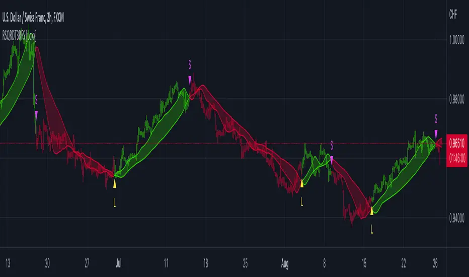
T3 Slope Variation [Loxx]T3 Slope Variation is an indicator that uses T3 moving average to calculate a slope that is then weighted to derive a signal.
The center line
The center line changes color depending on the value of the:
Slope
Signal line
Threshold
If the value is above a signal line (it is not visible on the chart) and the threshold is greater than the required, then the main trend becomes up. And reversed for the trend down.
Colors and style of the histogram
The colors and style of the histogram will be drawn if the value is at the right side, if the above described trend "agrees" with the value (above is green or below zero is red) and if the High is higher than the previous High or Low is lower than the previous low, then the according type of histogram is drawn.
What is the T3 moving average?
Better Moving Averages Tim Tillson
November 1, 1998
Tim Tillson is a software project manager at Hewlett-Packard, with degrees in Mathematics and Computer Science. He has privately traded options and equities for 15 years.
Introduction
"Digital filtering includes the process of smoothing, predicting, differentiating, integrating, separation of signals, and removal of noise from a signal. Thus many people who do such things are actually using digital filters without realizing that they are; being unacquainted with the theory, they neither understand what they have done nor the possibilities of what they might have done."
This quote from R. W. Hamming applies to the vast majority of indicators in technical analysis . Moving averages, be they simple, weighted, or exponential, are lowpass filters; low frequency components in the signal pass through with little attenuation, while high frequencies are severely reduced.
"Oscillator" type indicators (such as MACD , Momentum, Relative Strength Index ) are another type of digital filter called a differentiator.
Tushar Chande has observed that many popular oscillators are highly correlated, which is sensible because they are trying to measure the rate of change of the underlying time series, i.e., are trying to be the first and second derivatives we all learned about in Calculus.
We use moving averages (lowpass filters) in technical analysis to remove the random noise from a time series, to discern the underlying trend or to determine prices at which we will take action. A perfect moving average would have two attributes:
It would be smooth, not sensitive to random noise in the underlying time series. Another way of saying this is that its derivative would not spuriously alternate between positive and negative values.
It would not lag behind the time series it is computed from. Lag, of course, produces late buy or sell signals that kill profits.
The only way one can compute a perfect moving average is to have knowledge of the future, and if we had that, we would buy one lottery ticket a week rather than trade!
Having said this, we can still improve on the conventional simple, weighted, or exponential moving averages. Here's how:
Two Interesting Moving Averages
We will examine two benchmark moving averages based on Linear Regression analysis.
In both cases, a Linear Regression line of length n is fitted to price data.
I call the first moving average ILRS, which stands for Integral of Linear Regression Slope. One simply integrates the slope of a linear regression line as it is successively fitted in a moving window of length n across the data, with the constant of integration being a simple moving average of the first n points. Put another way, the derivative of ILRS is the linear regression slope. Note that ILRS is not the same as a SMA ( simple moving average ) of length n, which is actually the midpoint of the linear regression line as it moves across the data.
We can measure the lag of moving averages with respect to a linear trend by computing how they behave when the input is a line with unit slope. Both SMA (n) and ILRS(n) have lag of n/2, but ILRS is much smoother than SMA .
Our second benchmark moving average is well known, called EPMA or End Point Moving Average. It is the endpoint of the linear regression line of length n as it is fitted across the data. EPMA hugs the data more closely than a simple or exponential moving average of the same length. The price we pay for this is that it is much noisier (less smooth) than ILRS, and it also has the annoying property that it overshoots the data when linear trends are present.
However, EPMA has a lag of 0 with respect to linear input! This makes sense because a linear regression line will fit linear input perfectly, and the endpoint of the LR line will be on the input line.
These two moving averages frame the tradeoffs that we are facing. On one extreme we have ILRS, which is very smooth and has considerable phase lag. EPMA has 0 phase lag, but is too noisy and overshoots. We would like to construct a better moving average which is as smooth as ILRS, but runs closer to where EPMA lies, without the overshoot.
A easy way to attempt this is to split the difference, i.e. use (ILRS(n)+EPMA(n))/2. This will give us a moving average (call it IE /2) which runs in between the two, has phase lag of n/4 but still inherits considerable noise from EPMA. IE /2 is inspirational, however. Can we build something that is comparable, but smoother? Figure 1 shows ILRS, EPMA, and IE /2.
Filter Techniques
Any thoughtful student of filter theory (or resolute experimenter) will have noticed that you can improve the smoothness of a filter by running it through itself multiple times, at the cost of increasing phase lag.
There is a complementary technique (called twicing by J.W. Tukey) which can be used to improve phase lag. If L stands for the operation of running data through a low pass filter, then twicing can be described by:
L' = L(time series) + L(time series - L(time series))
That is, we add a moving average of the difference between the input and the moving average to the moving average. This is algebraically equivalent to:
2L-L(L)
This is the Double Exponential Moving Average or DEMA , popularized by Patrick Mulloy in TASAC (January/February 1994).
In our taxonomy, DEMA has some phase lag (although it exponentially approaches 0) and is somewhat noisy, comparable to IE /2 indicator.
We will use these two techniques to construct our better moving average, after we explore the first one a little more closely.
Fixing Overshoot
An n-day EMA has smoothing constant alpha=2/(n+1) and a lag of (n-1)/2.
Thus EMA (3) has lag 1, and EMA (11) has lag 5. Figure 2 shows that, if I am willing to incur 5 days of lag, I get a smoother moving average if I run EMA (3) through itself 5 times than if I just take EMA (11) once.
This suggests that if EPMA and DEMA have 0 or low lag, why not run fast versions (eg DEMA (3)) through themselves many times to achieve a smooth result? The problem is that multiple runs though these filters increase their tendency to overshoot the data, giving an unusable result. This is because the amplitude response of DEMA and EPMA is greater than 1 at certain frequencies, giving a gain of much greater than 1 at these frequencies when run though themselves multiple times. Figure 3 shows DEMA (7) and EPMA(7) run through themselves 3 times. DEMA^3 has serious overshoot, and EPMA^3 is terrible.
The solution to the overshoot problem is to recall what we are doing with twicing:
DEMA (n) = EMA (n) + EMA (time series - EMA (n))
The second term is adding, in effect, a smooth version of the derivative to the EMA to achieve DEMA . The derivative term determines how hot the moving average's response to linear trends will be. We need to simply turn down the volume to achieve our basic building block:
EMA (n) + EMA (time series - EMA (n))*.7;
This is algebraically the same as:
EMA (n)*1.7-EMA( EMA (n))*.7;
I have chosen .7 as my volume factor, but the general formula (which I call "Generalized Dema") is:
GD (n,v) = EMA (n)*(1+v)-EMA( EMA (n))*v,
Where v ranges between 0 and 1. When v=0, GD is just an EMA , and when v=1, GD is DEMA . In between, GD is a cooler DEMA . By using a value for v less than 1 (I like .7), we cure the multiple DEMA overshoot problem, at the cost of accepting some additional phase delay. Now we can run GD through itself multiple times to define a new, smoother moving average T3 that does not overshoot the data:
T3(n) = GD ( GD ( GD (n)))
In filter theory parlance, T3 is a six-pole non-linear Kalman filter. Kalman filters are ones which use the error (in this case (time series - EMA (n)) to correct themselves. In Technical Analysis , these are called Adaptive Moving Averages; they track the time series more aggressively when it is making large moves.
Included
Alets
Signals
Bar coloring
Loxx's Expanded Source Types
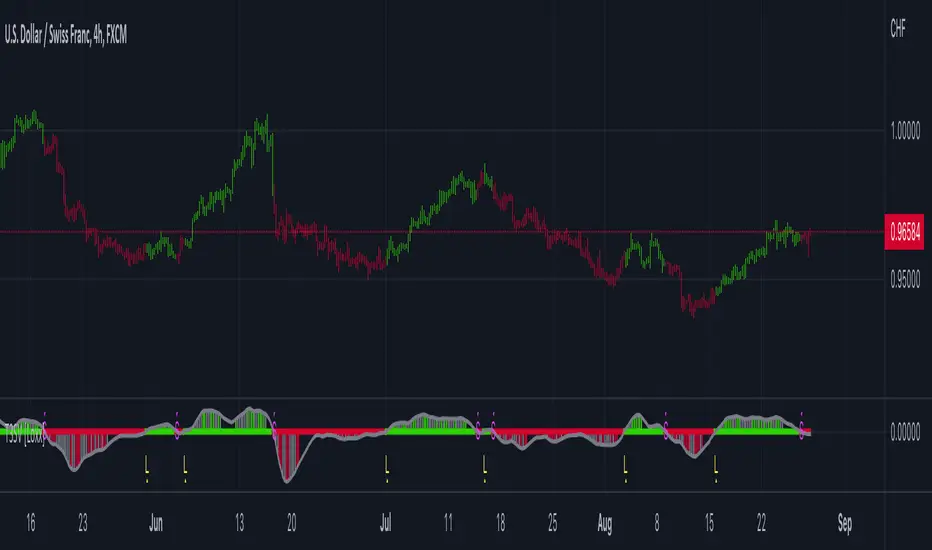
Multi T3 Slopes [Loxx]Multi T3 Slopes is an indicator that checks slopes of 5 (different period) T3 Moving Averages and adds them up to show overall trend. To us this, check for color changes from red to green where there is no red if green is larger than red and there is no red when red is larger than green. When red and green both show up, its a sign of chop.
What is the T3 moving average?
Better Moving Averages Tim Tillson
November 1, 1998
Tim Tillson is a software project manager at Hewlett-Packard, with degrees in Mathematics and Computer Science. He has privately traded options and equities for 15 years.
Introduction
"Digital filtering includes the process of smoothing, predicting, differentiating, integrating, separation of signals, and removal of noise from a signal. Thus many people who do such things are actually using digital filters without realizing that they are; being unacquainted with the theory, they neither understand what they have done nor the possibilities of what they might have done."
This quote from R. W. Hamming applies to the vast majority of indicators in technical analysis . Moving averages, be they simple, weighted, or exponential, are lowpass filters; low frequency components in the signal pass through with little attenuation, while high frequencies are severely reduced.
"Oscillator" type indicators (such as MACD , Momentum, Relative Strength Index ) are another type of digital filter called a differentiator.
Tushar Chande has observed that many popular oscillators are highly correlated, which is sensible because they are trying to measure the rate of change of the underlying time series, i.e., are trying to be the first and second derivatives we all learned about in Calculus.
We use moving averages (lowpass filters) in technical analysis to remove the random noise from a time series, to discern the underlying trend or to determine prices at which we will take action. A perfect moving average would have two attributes:
It would be smooth, not sensitive to random noise in the underlying time series. Another way of saying this is that its derivative would not spuriously alternate between positive and negative values.
It would not lag behind the time series it is computed from. Lag, of course, produces late buy or sell signals that kill profits.
The only way one can compute a perfect moving average is to have knowledge of the future, and if we had that, we would buy one lottery ticket a week rather than trade!
Having said this, we can still improve on the conventional simple, weighted, or exponential moving averages. Here's how:
Two Interesting Moving Averages
We will examine two benchmark moving averages based on Linear Regression analysis.
In both cases, a Linear Regression line of length n is fitted to price data.
I call the first moving average ILRS, which stands for Integral of Linear Regression Slope. One simply integrates the slope of a linear regression line as it is successively fitted in a moving window of length n across the data, with the constant of integration being a simple moving average of the first n points. Put another way, the derivative of ILRS is the linear regression slope. Note that ILRS is not the same as a SMA ( simple moving average ) of length n, which is actually the midpoint of the linear regression line as it moves across the data.
We can measure the lag of moving averages with respect to a linear trend by computing how they behave when the input is a line with unit slope. Both SMA (n) and ILRS(n) have lag of n/2, but ILRS is much smoother than SMA .
Our second benchmark moving average is well known, called EPMA or End Point Moving Average. It is the endpoint of the linear regression line of length n as it is fitted across the data. EPMA hugs the data more closely than a simple or exponential moving average of the same length. The price we pay for this is that it is much noisier (less smooth) than ILRS, and it also has the annoying property that it overshoots the data when linear trends are present.
However, EPMA has a lag of 0 with respect to linear input! This makes sense because a linear regression line will fit linear input perfectly, and the endpoint of the LR line will be on the input line.
These two moving averages frame the tradeoffs that we are facing. On one extreme we have ILRS, which is very smooth and has considerable phase lag. EPMA has 0 phase lag, but is too noisy and overshoots. We would like to construct a better moving average which is as smooth as ILRS, but runs closer to where EPMA lies, without the overshoot.
A easy way to attempt this is to split the difference, i.e. use (ILRS(n)+EPMA(n))/2. This will give us a moving average (call it IE /2) which runs in between the two, has phase lag of n/4 but still inherits considerable noise from EPMA. IE /2 is inspirational, however. Can we build something that is comparable, but smoother? Figure 1 shows ILRS, EPMA, and IE /2.
Filter Techniques
Any thoughtful student of filter theory (or resolute experimenter) will have noticed that you can improve the smoothness of a filter by running it through itself multiple times, at the cost of increasing phase lag.
There is a complementary technique (called twicing by J.W. Tukey) which can be used to improve phase lag. If L stands for the operation of running data through a low pass filter, then twicing can be described by:
L' = L(time series) + L(time series - L(time series))
That is, we add a moving average of the difference between the input and the moving average to the moving average. This is algebraically equivalent to:
2L-L(L)
This is the Double Exponential Moving Average or DEMA , popularized by Patrick Mulloy in TASAC (January/February 1994).
In our taxonomy, DEMA has some phase lag (although it exponentially approaches 0) and is somewhat noisy, comparable to IE /2 indicator.
We will use these two techniques to construct our better moving average, after we explore the first one a little more closely.
Fixing Overshoot
An n-day EMA has smoothing constant alpha=2/(n+1) and a lag of (n-1)/2.
Thus EMA (3) has lag 1, and EMA (11) has lag 5. Figure 2 shows that, if I am willing to incur 5 days of lag, I get a smoother moving average if I run EMA (3) through itself 5 times than if I just take EMA (11) once.
This suggests that if EPMA and DEMA have 0 or low lag, why not run fast versions (eg DEMA (3)) through themselves many times to achieve a smooth result? The problem is that multiple runs though these filters increase their tendency to overshoot the data, giving an unusable result. This is because the amplitude response of DEMA and EPMA is greater than 1 at certain frequencies, giving a gain of much greater than 1 at these frequencies when run though themselves multiple times. Figure 3 shows DEMA (7) and EPMA(7) run through themselves 3 times. DEMA^3 has serious overshoot, and EPMA^3 is terrible.
The solution to the overshoot problem is to recall what we are doing with twicing:
DEMA (n) = EMA (n) + EMA (time series - EMA (n))
The second term is adding, in effect, a smooth version of the derivative to the EMA to achieve DEMA . The derivative term determines how hot the moving average's response to linear trends will be. We need to simply turn down the volume to achieve our basic building block:
EMA (n) + EMA (time series - EMA (n))*.7;
This is algebraically the same as:
EMA (n)*1.7-EMA( EMA (n))*.7;
I have chosen .7 as my volume factor, but the general formula (which I call "Generalized Dema") is:
GD (n,v) = EMA (n)*(1+v)-EMA( EMA (n))*v,
Where v ranges between 0 and 1. When v=0, GD is just an EMA , and when v=1, GD is DEMA . In between, GD is a cooler DEMA . By using a value for v less than 1 (I like .7), we cure the multiple DEMA overshoot problem, at the cost of accepting some additional phase delay. Now we can run GD through itself multiple times to define a new, smoother moving average T3 that does not overshoot the data:
T3(n) = GD ( GD ( GD (n)))
In filter theory parlance, T3 is a six-pole non-linear Kalman filter. Kalman filters are ones which use the error (in this case (time series - EMA (n)) to correct themselves. In Technical Analysis , these are called Adaptive Moving Averages; they track the time series more aggressively when it is making large moves.
Included
Signals: long, short, continuation long, continuation short.
Alerts
Bar coloring
Loxx's expanded source types
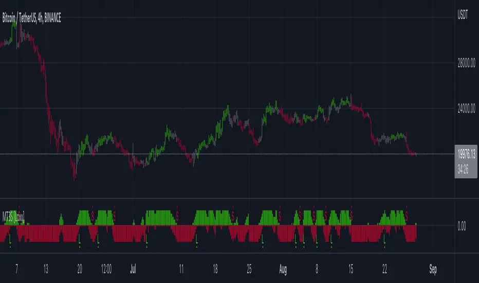
T3 Volatility Quality Index (VQI) w/ DSL & Pips Filtering [Loxx]T3 Volatility Quality Index (VQI) w/ DSL & Pips Filtering is a VQI indicator that uses T3 smoothing and discontinued signal lines to determine breakouts and breakdowns. This also allows filtering by pips.***
What is the Volatility Quality Index ( VQI )?
The idea behind the volatility quality index is to point out the difference between bad and good volatility in order to identify better trade opportunities in the market. This forex indicator works using the True Range algorithm in combination with the open, close, high and low prices.
What are DSL Discontinued Signal Line?
A lot of indicators are using signal lines in order to determine the trend (or some desired state of the indicator) easier. The idea of the signal line is easy : comparing the value to it's smoothed (slightly lagging) state, the idea of current momentum/state is made.
Discontinued signal line is inheriting that simple signal line idea and it is extending it : instead of having one signal line, more lines depending on the current value of the indicator.
"Signal" line is calculated the following way :
When a certain level is crossed into the desired direction, the EMA of that value is calculated for the desired signal line
When that level is crossed into the opposite direction, the previous "signal" line value is simply "inherited" and it becomes a kind of a level
This way it becomes a combination of signal lines and levels that are trying to combine both the good from both methods.
In simple terms, DSL uses the concept of a signal line and betters it by inheriting the previous signal line's value & makes it a level.
What is the T3 moving average?
Better Moving Averages Tim Tillson
November 1, 1998
Tim Tillson is a software project manager at Hewlett-Packard, with degrees in Mathematics and Computer Science. He has privately traded options and equities for 15 years.
Introduction
"Digital filtering includes the process of smoothing, predicting, differentiating, integrating, separation of signals, and removal of noise from a signal. Thus many people who do such things are actually using digital filters without realizing that they are; being unacquainted with the theory, they neither understand what they have done nor the possibilities of what they might have done."
This quote from R. W. Hamming applies to the vast majority of indicators in technical analysis . Moving averages, be they simple, weighted, or exponential, are lowpass filters; low frequency components in the signal pass through with little attenuation, while high frequencies are severely reduced.
"Oscillator" type indicators (such as MACD , Momentum, Relative Strength Index ) are another type of digital filter called a differentiator.
Tushar Chande has observed that many popular oscillators are highly correlated, which is sensible because they are trying to measure the rate of change of the underlying time series, i.e., are trying to be the first and second derivatives we all learned about in Calculus.
We use moving averages (lowpass filters) in technical analysis to remove the random noise from a time series, to discern the underlying trend or to determine prices at which we will take action. A perfect moving average would have two attributes:
It would be smooth, not sensitive to random noise in the underlying time series. Another way of saying this is that its derivative would not spuriously alternate between positive and negative values.
It would not lag behind the time series it is computed from. Lag, of course, produces late buy or sell signals that kill profits.
The only way one can compute a perfect moving average is to have knowledge of the future, and if we had that, we would buy one lottery ticket a week rather than trade!
Having said this, we can still improve on the conventional simple, weighted, or exponential moving averages. Here's how:
Two Interesting Moving Averages
We will examine two benchmark moving averages based on Linear Regression analysis.
In both cases, a Linear Regression line of length n is fitted to price data.
I call the first moving average ILRS, which stands for Integral of Linear Regression Slope. One simply integrates the slope of a linear regression line as it is successively fitted in a moving window of length n across the data, with the constant of integration being a simple moving average of the first n points. Put another way, the derivative of ILRS is the linear regression slope. Note that ILRS is not the same as a SMA ( simple moving average ) of length n, which is actually the midpoint of the linear regression line as it moves across the data.
We can measure the lag of moving averages with respect to a linear trend by computing how they behave when the input is a line with unit slope. Both SMA (n) and ILRS(n) have lag of n/2, but ILRS is much smoother than SMA .
Our second benchmark moving average is well known, called EPMA or End Point Moving Average. It is the endpoint of the linear regression line of length n as it is fitted across the data. EPMA hugs the data more closely than a simple or exponential moving average of the same length. The price we pay for this is that it is much noisier (less smooth) than ILRS, and it also has the annoying property that it overshoots the data when linear trends are present.
However, EPMA has a lag of 0 with respect to linear input! This makes sense because a linear regression line will fit linear input perfectly, and the endpoint of the LR line will be on the input line.
These two moving averages frame the tradeoffs that we are facing. On one extreme we have ILRS, which is very smooth and has considerable phase lag. EPMA has 0 phase lag, but is too noisy and overshoots. We would like to construct a better moving average which is as smooth as ILRS, but runs closer to where EPMA lies, without the overshoot.
A easy way to attempt this is to split the difference, i.e. use (ILRS(n)+EPMA(n))/2. This will give us a moving average (call it IE /2) which runs in between the two, has phase lag of n/4 but still inherits considerable noise from EPMA. IE /2 is inspirational, however. Can we build something that is comparable, but smoother? Figure 1 shows ILRS, EPMA, and IE /2.
Filter Techniques
Any thoughtful student of filter theory (or resolute experimenter) will have noticed that you can improve the smoothness of a filter by running it through itself multiple times, at the cost of increasing phase lag.
There is a complementary technique (called twicing by J.W. Tukey) which can be used to improve phase lag. If L stands for the operation of running data through a low pass filter, then twicing can be described by:
L' = L(time series) + L(time series - L(time series))
That is, we add a moving average of the difference between the input and the moving average to the moving average. This is algebraically equivalent to:
2L-L(L)
This is the Double Exponential Moving Average or DEMA , popularized by Patrick Mulloy in TASAC (January/February 1994).
In our taxonomy, DEMA has some phase lag (although it exponentially approaches 0) and is somewhat noisy, comparable to IE /2 indicator.
We will use these two techniques to construct our better moving average, after we explore the first one a little more closely.
Fixing Overshoot
An n-day EMA has smoothing constant alpha=2/(n+1) and a lag of (n-1)/2.
Thus EMA (3) has lag 1, and EMA (11) has lag 5. Figure 2 shows that, if I am willing to incur 5 days of lag, I get a smoother moving average if I run EMA (3) through itself 5 times than if I just take EMA (11) once.
This suggests that if EPMA and DEMA have 0 or low lag, why not run fast versions (eg DEMA (3)) through themselves many times to achieve a smooth result? The problem is that multiple runs though these filters increase their tendency to overshoot the data, giving an unusable result. This is because the amplitude response of DEMA and EPMA is greater than 1 at certain frequencies, giving a gain of much greater than 1 at these frequencies when run though themselves multiple times. Figure 3 shows DEMA (7) and EPMA(7) run through themselves 3 times. DEMA^3 has serious overshoot, and EPMA^3 is terrible.
The solution to the overshoot problem is to recall what we are doing with twicing:
DEMA (n) = EMA (n) + EMA (time series - EMA (n))
The second term is adding, in effect, a smooth version of the derivative to the EMA to achieve DEMA . The derivative term determines how hot the moving average's response to linear trends will be. We need to simply turn down the volume to achieve our basic building block:
EMA (n) + EMA (time series - EMA (n))*.7;
This is algebraically the same as:
EMA (n)*1.7-EMA( EMA (n))*.7;
I have chosen .7 as my volume factor, but the general formula (which I call "Generalized Dema") is:
GD (n,v) = EMA (n)*(1+v)-EMA( EMA (n))*v,
Where v ranges between 0 and 1. When v=0, GD is just an EMA , and when v=1, GD is DEMA . In between, GD is a cooler DEMA . By using a value for v less than 1 (I like .7), we cure the multiple DEMA overshoot problem, at the cost of accepting some additional phase delay. Now we can run GD through itself multiple times to define a new, smoother moving average T3 that does not overshoot the data:
T3(n) = GD ( GD ( GD (n)))
In filter theory parlance, T3 is a six-pole non-linear Kalman filter. Kalman filters are ones which use the error (in this case (time series - EMA (n)) to correct themselves. In Technical Analysis , these are called Adaptive Moving Averages; they track the time series more aggressively when it is making large moves.
Included
Signals
Alerts
Related indicators
Zero-line Volatility Quality Index (VQI)
Volatility Quality Index w/ Pips Filtering
Variety Moving Average Waddah Attar Explosion (WAE)
***This indicator is tuned to Forex. If you want to make it useful for other tickers, you must change the pip filtering value to match the asset. This means that for BTC, for example, you likely need to use a value of 10,000 or more for pips filter.
