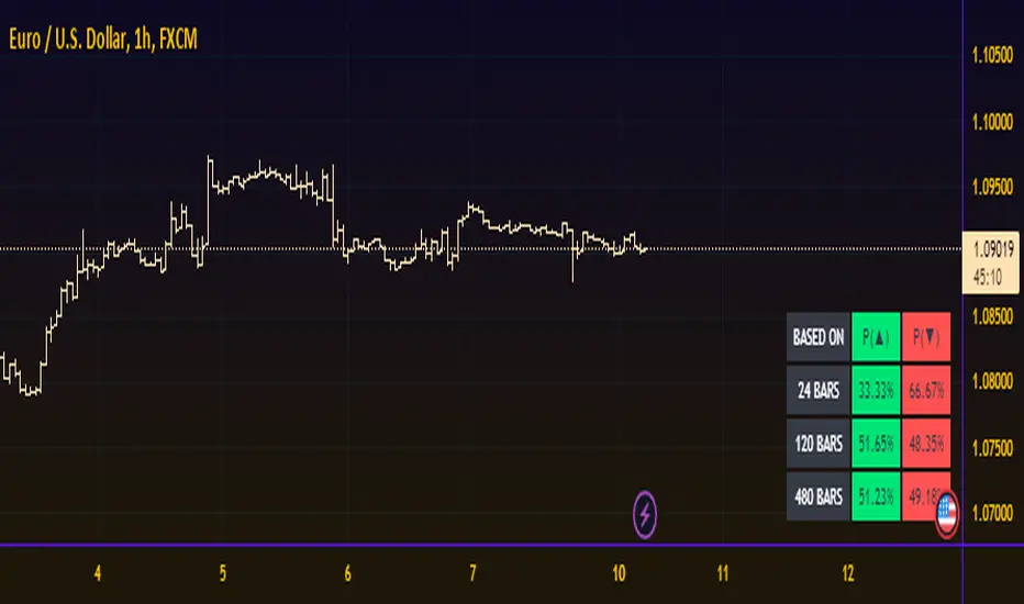
Probability TableThe script is inspired by user NickbarComb, I suggested checking out his Price Convergence script.
Basically, this script plots a table containing the probability of the current candle closing either higher or lower based on user-define past period.
Hope that it will be helpful.
חפש סקריפטים עבור "Table"
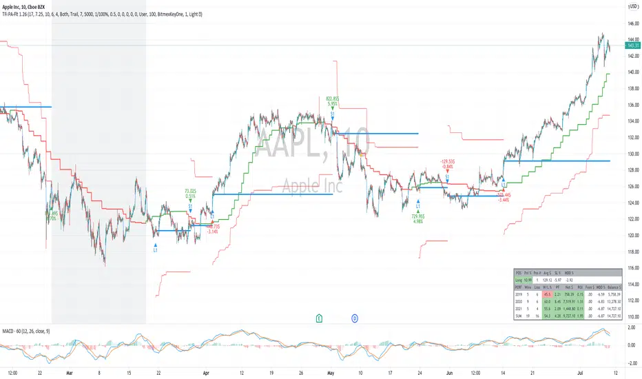
TFi Price Action Resampling Filter V1 - FULLThe script is resampling the price based on its range/price-action and creates an alternative filter to smoothen price movements.
Overview of features:
Optional stop-loss
Optional flags to control the position entry
Optional flags to control the position exit
Built-in backtesting engine with start balance, position size and pyramiding; each year will be evaluated separately
Inputs for a percentage entry and exit slippage, entry/exit and daily funding fees
Configurable alerts, which follow the exact position of the entry/exit marker
Alert messages contain predefined trading instruction to execute orders via Alertatron or TradeFab's proprietary trading server, or can be defined by the user
The script renders a performance/status table, which shows the current position status and result of the built-in trading simulation results.
It shows the following statistic values:
Current position PnL - also background turns green if position is in profit and red if in loss
Average entry price and number of positions
Current percentage distance to the optional stop-loss level
Current Maximum Draw Down
Number of wins and losses and the win/loss ratio per year and overall
Profit and loss amount, paid fees per year and overall
Profit-ratio and Maximum Draw Down per year and overall
Balance and ROI per year and overall
MTF Price/Volume % [Anan]Hello friends,
This is a multi-timeframe table with these features:
Display price change percentage compared with the last timeframe candle close.
Display price change percentage compared with the last timeframe candle close MA.
Displays change percentage compared with the last timeframe candle volume.
Displays change percentage compared with the last timeframe candle volume MA.
Change type/length of MA for Price/Volume.
Full control of Panel position and size.
Full control of displaying any row or column.

Average Daily Range TableThis is the last script to complete Vladimir Poltoratskiy's setup found in his books.
Poltoratskiy argues that you should not take any fractal corridors higher than 50% of the Average Daily Range. To be honest, even 40% is a lot, because then, your target will be 160% ADR away from your entry and one "fracture" just can't be enough to predict moves this big.
I chose a table to visually represent the indicator because it doesn't change its value during the day. It takes far less room on the chart.
There are also two simple moving averages. You may use the as an indicator if the relative volatility as of late is extremely low and in that case, perhaps, expect an increase in the coming days. They are applied to the Average Daily Range, not one day range!

Relative Volume TableRelative Volume Table in percent. So 400% RVol means, today's volume is 4x compared to avg volume for the length you selected.
1. When chart resolution is Daily or Intraday (D, 4H, 1H, 5min, etc), Relative Volume shows value based on DAILY.
2. When resolution is changed to Weekly or Monthly, then Relative Volume shows corresponding value. i.e. Weekly shows weekly relative volume of this week compared to past 'N' weeks. Likewise for Monthly. You would see change in label name. Like, Weekly chart shows W_RVol (Weekly Relative Volume). Likewise, Daily & Intraday shows D_RVol. Monthly shows M_RVol (Monthly Relative Volume).
3. Added a plot (by default hidden) for this specific reason: When you move the cursor to focus specific candle, then Indicator Value displays relative volume of that specific candle. This applies to Intraday as well. So if you're in 1HR chart and move the cursor to a specific candle, Indicator Value shows relative volume for that specific candlestick bar.
Hope you find this useful.

PAC newThis indicator will alert you when a candle goes above or below the price action channel (PAC) but only on the first or second candle after a colour change in candle.
When price is above the price action channel that is a bullish sign, when price is below the PAC that is a bearish sign.
The idea is that a sudden change in price is a cause to investigate further price action moving in that direction so the indicator aims to identify reversal
Scalping strategy that works on 5 min chart and aims to gain 10 pips. Do not act on every signal. Further investigation is required, for example by looking at RSI oversolf and overbought levels. For example, at an oversold area, a buy signal is more valid

Table: Forex Central Bank Interest RatesThis tool shows CB Interest Rates for USD, JPY, CAD, CHF, EUR, GBP, NZD, AUD - basically all the majors.
Use override and input your own value if it is changed and I haven't updated the script yet.

Month/Month Percentage % Change, Historical; Seasonal TendencyTable of monthly % changes in Average Price over the last 10 years (or the 10 yrs prior to input year).
Useful for gauging seasonal tendencies of an asset; backtesting monthly volatility and bullish/bearish tendency.
~~User Inputs~~
Choose measure of average: sma(close), sma(ohlc4), vwap(close), vwma(close).
Show last 10yrs, with 10yr average % change, or to just show single year.
Chose input year; with the indicator auto calculating the prior 10 years.
Choose color for labels and size for labels; choose +Ve value color and -Ve value color.
Set 'Daily bars in month': 21 for Forex/Commodities/Indices; 30 for Crypto.
Set precision: decimal places
~~notes~~
-designed for use on Daily timeframe (tradingview is buggy on monthly timeframe calculations, and less precise on weekly timeframe calculations).
-where Current month of year has not occurred yet, will print 9yr average.
-calculates the average change of displayed month compared to the previous month: i.e. Jan22 value represents whole of Jan22 compared to whole of Dec21.
-table displays on the chart over the input year; so for ES, with 2010 selected; shows values from 2001-2010, displaying across 2010-2011 on the chart.
-plots on seperate right hand side scale, so can be shrunk and dragged vertically.
-thanks to @gabx11 for the suggestion which inspired me to write this

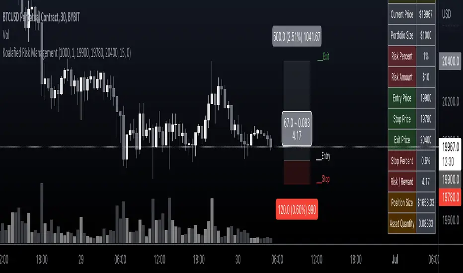
Koalafied Risk ManagementTables and labels/lines showing trade levels and risk/reward. Use to manage trade risk compared to portfolio size.
Initial design optimised for tickers denominated against USD.
Multi-Session High/Low Trackertable that shows rth eth and full weekly range high and low with range difference from high and low

Table ATH and DayQuotes in the middle of a chartJust important things at a glance ..
AlltimeHigh and Daily High/Low

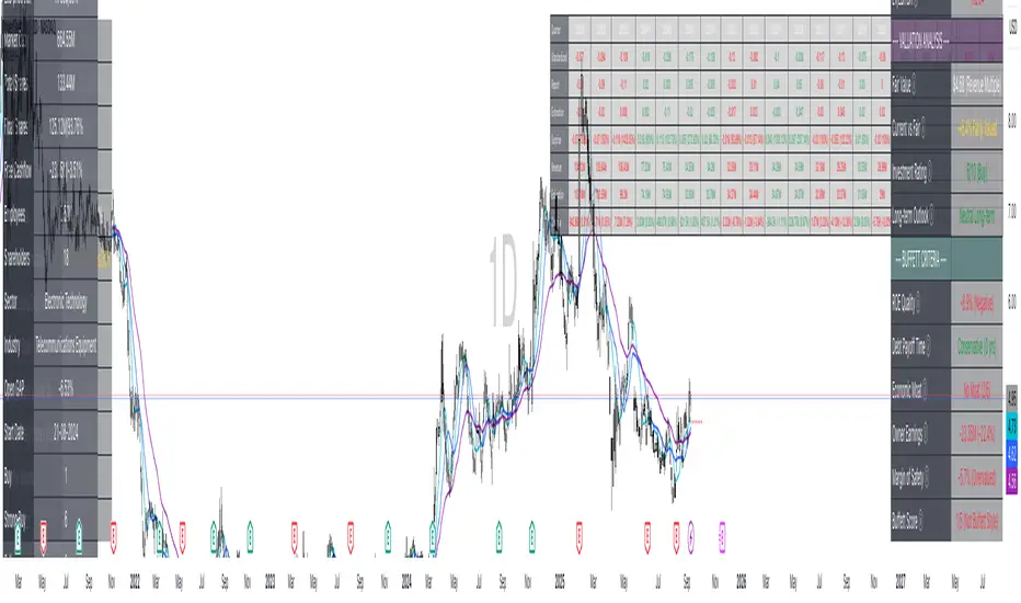
Stocker++Stocker++ Comprehensive Documentation
Overview
Stocker++ is an advanced stock analysis indicator that combines technical trend analysis with fundamental company data to provide comprehensive investment insights. This all-in-one tool displays multiple moving averages for trend identification and presents detailed financial information through organized data tables, helping investors make informed decisions based on both price action and company fundamentals.
Key Features
1. Customizable Moving Averages
Up to 6 configurable moving averages (MA1-MA6)
Choice between Simple Moving Average (SMA) and Exponential Moving Average (EMA)
Individual color customization for each MA
Adjustable lengths, timeframes, and visibility toggles
Default setup includes 10, 20, and 50-period MAs for short to medium-term trend analysis
2. Risk Management Table
Displays critical position sizing and risk calculations:
Account Size: Your total trading capital
Risk Money: Dollar amount and percentage at risk per trade
Stop Loss: Calculated using either ATR or Low of Day
Shares to Buy: Optimal position size based on risk parameters
Position Size: Total dollar amount and percentage of account
Max Allowed Position: Maximum position based on liquidity constraints (Daily Volume ÷ 200)
Min Required Daily Vol: Minimum liquidity needed for your position size
Liquidity Ratio: How many times over the minimum liquidity requirement
Average Daily Volume ($): 20-day average dollar volume
Average Daily Shares Volume: 20-day average share volume
Relative Volume: Current volume compared to 20-day average
Volume Buzz: Percentage increase/decrease from average volume
3. Company Info Table
Essential company metrics and market data:
Change: Daily price change in dollars
ATR: Average True Range for volatility measurement
ADR: Average Daily Range percentage
LoD price/dist: Low of Day price and distance percentage
Market Cap: Total market capitalization
Total Shares: Outstanding shares
Float Shares: Tradeable shares and percentage of total
Free Cashflow: Cash generation and percentage of market cap
Employees: Total employee count
Shareholders: Number of shareholders
Sector/Industry: Business classification
Open GAP: Gap percentage from previous day
Analyst Ratings: Buy/Strong Buy/Hold/Sell/Strong Sell recommendations with totals
4. Earnings Table
Quarterly earnings history displaying:
Quarter: Year/Month of earnings
Standardized: Standardized EPS
Report: Actual reported EPS
Estimation: Analyst consensus estimate
Surprise: Beat/miss amount and percentage
Revenue: Actual quarterly revenue
Estimation: Revenue estimates
Surprise: Revenue beat/miss with percentage
Color-coded results (green for beats, red for misses)
5. Financial Analysis Table
Comprehensive fundamental analysis across multiple sections:
Income Statement:
Revenue (Quarterly)
Gross Profit with margin percentage
Operating Income with margin
Net Income with margin
Earnings Per Share (EPS)
Balance Sheet:
Total Assets
Total Liabilities
Shareholders Equity
Cash & Equivalents
Total Debt
Debt/Equity Ratio
Valuation Metrics:
Market Cap
Enterprise Value
EV/Revenue
Price/Book Ratio
Book Value per Share
Return on Equity (ROE)
Return on Assets (ROA)
Key Multipliers:
P/E Ratio
P/S Ratio
PEG Ratio
EV/EBITDA
Valuation Analysis:
Fair Value calculation using multiple methods
Current vs Fair Value percentage
Investment Rating (0-10 scale)
Long-term Outlook assessment
Warren Buffett Criteria:
ROE Quality (>15% target)
Debt Payoff Time (<3 years ideal)
Economic Moat score (0-6)
Owner Earnings with margin
Margin of Safety (>25% target)
Overall Buffett Score (0-5)
Settings Configuration
Moving Average Settings
Enable/Disable: Toggle each MA on/off
MA Type: Choose SMA or EMA for each line
Length: Set period for each MA (default: 10, 20, 50, 100, 150, 200)
Timeframe: Set specific timeframe for each MA
Colors: Customize each MA line color
Table Settings
Each table includes:
Show/Hide Toggle: Enable or disable individual tables
Position: Choose from 6 screen positions
Text Size: Auto, Tiny, Small, Normal, Large, or Huge
Colors: Customize table background, highlight, and text colors
Risk Management Settings
Account Size: Your trading capital
Risk Per Trade (%): Percentage to risk per position
Position Multiplier: Adjustment factor for position sizing
Stop Loss Level: Choose between ADR or Low of Day
ADR/ATR Length: Periods for volatility calculations
Usage Tips
Trend Analysis: Use moving averages to identify trend direction and strength. Price above all MAs suggests uptrend.
Position Sizing: Use the Risk Management table to calculate proper position size based on your risk tolerance.
Liquidity Check: Ensure the Liquidity Ratio is >1 (preferably >2) before entering large positions.
Earnings Analysis: Review earnings history for consistency and trend. Look for companies that consistently beat estimates.
Buffett Score: A score of 4-5 indicates a potential long-term value investment following Warren Buffett's principles.
Investment Rating: Scores above 7 suggest strong investment potential, while below 4 indicates caution.
Important Notes
Designed exclusively for stock market analysis
All recommendations are for educational purposes only
Best used in conjunction with personal research and risk tolerance
Data updates in real-time during market hours
Some financial metrics may not be available for all stocks (particularly pre-revenue companies)
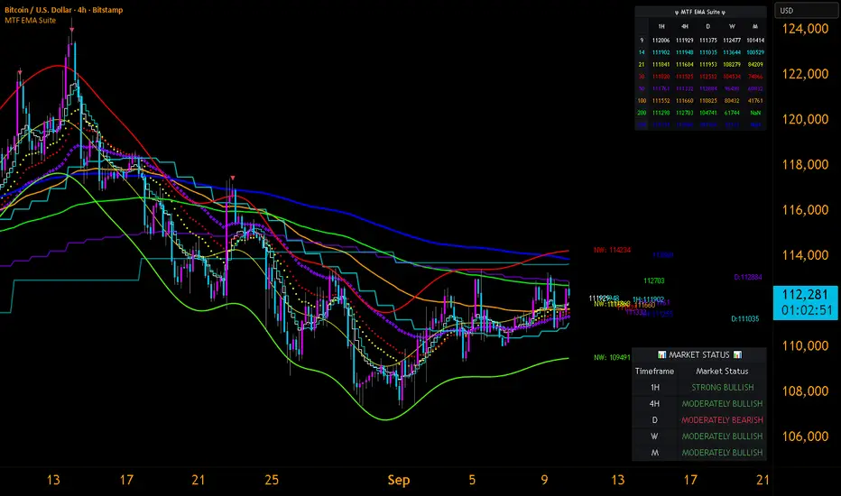
Multi-Timeframe EMA Analysis SuiteThis comprehensive multi-timeframe moving average analysis tool provides systematic trend evaluation across five configurable timeframes with advanced kernel regression envelope technology for dynamic boundary detection.
Core Innovation - Multi-Timeframe EMA System:
The primary functionality displays multiple exponential moving averages (9, 21, 30, 50, 100, 200), weighted moving average (14), and simple moving average (200) across customizable timeframes including 1H, 4H, Daily, Weekly, and Monthly periods. Each timeframe and moving average can be individually enabled or disabled based on analysis requirements.
Advanced Features:
Intelligent label positioning algorithms with automatic overlap prevention across multiple timeframes
Dynamic offset calculation maintaining readability when price levels converge
Comprehensive data table displaying all moving average values with color-coded formatting
Real-time market status evaluation categorizing conditions from "Strong Bullish" to "Strong Bearish"
Performance-optimized rendering with adjustable detail controls
Technical Implementation:
Built using Pine Script v6 with optimized multi-timeframe security requests through tuple-based data retrieval
The system implements efficient memory management and dynamic table systems for responsive chart performance during complex multi-timeframe calculations
Original developments include intelligent label spacing algorithms, dynamic offset management across timeframes, and comprehensive market status evaluation logic using moving average alignment principles
Enhanced Envelope System:
Incorporates and significantly extends the kernel regression envelope concept originally developed by LuxAlgo in their Nadaraya-Watson Envelope indicator. The mathematical foundation uses Gaussian weighting functions with substantial implementation improvements:
Complete redesign using optimized polyline rendering system for superior performance
Addition of center line calculation and visualization not present in the original
Performance optimization controls with adjustable detail levels
Enhanced label management with real-time value displays
Seamless integration with multi-timeframe analysis capabilities
Configuration Options:
Complete customization including timeframe selection, moving average lengths, envelope parameters, label positioning, table sizing, and visual styling. Users can create personalized analysis setups tailored to specific trading timeframes and analytical preferences.
Practical Applications:
Suitable for trend confirmation across multiple timeframes, identification of dynamic support and resistance levels, multi-timeframe market structure analysis, and systematic market direction evaluation
The combination of traditional moving averages with adaptive envelope boundaries provides both classical technical analysis and modern algorithmic boundary detection
Usage Instructions:
Enable desired timeframes and moving averages based on your analysis period
The envelope provides dynamic support/resistance levels while moving averages indicate directional bias. Use repainting mode for current analysis or non-repainting mode for consistent historical signals. Adjust performance settings based on system requirements and analysis detail needs
Educational Purpose:
This indicator is designed for educational and analytical purposes. Users should conduct thorough testing and validation before incorporating this tool into trading decisions.
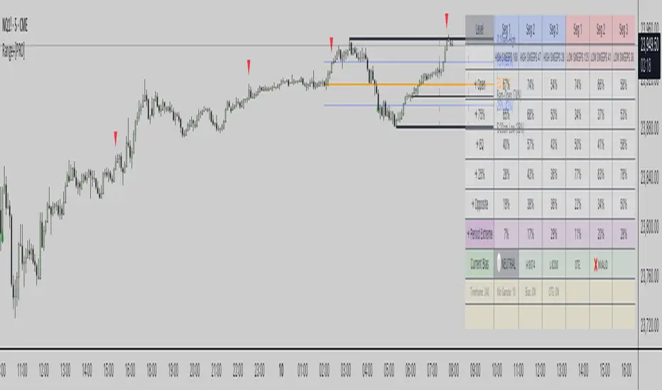
Range Stats with Sweeps + Time Analysis + BiasRange Stats with Sweeps + Time Analysis + Bias
Advanced range-based trading analysis with comprehensive sweep detection, time-based probability modeling, and intelligent bias calculation for institutional-grade market insights.
Overview
Range Stats with Sweeps + Time Analysis + Bias is a sophisticated Pine Script indicator designed for professional traders who demand precision in range-based market analysis. This comprehensive tool combines traditional range level analysis with advanced sweep detection algorithms, time-based probability modeling, and dynamic bias calculation to provide institutional-quality insights into market behavior patterns.
Core Features
Multi-Timeframe Range Analysis
Automatic or manual timeframe selection with intelligent defaults
Comprehensive range level calculation including High, Low, Open, 75%, EQ (50%), and 25% retracements
Dynamic period detection supporting both traditional timeframes and custom session-based analysis
Real-time range updates with historical data preservation
Advanced Sweep Detection System
Configurable sweep validation with customizable bar confirmation periods
Optional wick-based sweep requirements for enhanced precision
Segment-based sweep tracking dividing periods into three analytical zones
Real-time sweep markers with probability-enhanced labeling
Comprehensive Bias Calculation Framework
Intelligent range bias determination based on price action relative to range boundaries
Dynamic bias tracking with bullish, bearish, and neutral state identification
Historical bias performance statistics with hit rate analysis
Optimal Trade Entry (OTE) box generation based on current bias and displacement analysis
Time-Based Probability Analysis
Formation time tracking for high and low levels with customizable time buckets
Sweep probability calculation based on exact formation timing
Multiple time range displays including Full 24H, Extended Trading, US Market, EU Market, and Asia Market sessions
Custom session configuration with intelligent session-based level detection
Professional Visualization System
Customizable line styles, colors, and transparency settings for all range levels
Segment projection lines for period structure visualization
Comprehensive probability tables with real-time statistics
Time-enhanced labels showing formation times and sweep probabilities
Technical Implementation
Range Detection Logic
The system employs sophisticated algorithms to identify range boundaries using either traditional timeframe-based detection or custom session-based analysis. Range levels are calculated with mathematical precision, providing 75%, 50%, and 25% retracement levels based on period high-low ranges.
Sweep Analysis Framework
Advanced sweep detection monitors price action for liquidity grabs above highs and below lows, with configurable validation periods ensuring sweep authenticity. The system tracks sweep occurrences across three distinct period segments, enabling granular probability analysis.
Bias Calculation Engine
The intelligent bias system analyzes price behavior relative to range boundaries, considering factors such as wick interactions, close positioning, and directional momentum. This generates dynamic bias signals that adapt to changing market conditions.
Time-Based Modeling
Sophisticated time bucket analysis tracks formation times for range extremes, building comprehensive probability models that identify optimal trading windows based on historical performance patterns.
Configuration Options
Core Settings
Automatic or manual timeframe selection with comprehensive options
Global timezone support with major market timezone presets
Configurable label sizing and time format preferences
Advanced sweep validation parameters with wick-based options
Range Level Customization
Individual control over all range level displays and styling
Custom color schemes with transparency controls
Line style selection including solid, dashed, and dotted options
Adjustable line widths for enhanced visual hierarchy
Advanced Features
Segment projection line configuration for period structure analysis
Bias calculation toggle with OTE box generation
Sweep extreme probability tracking with period extreme analysis
Comprehensive sweep marker system with probability labeling
Time Analysis Configuration
Multiple time bucket options including 20-minute, 1-hour, 2-hour, and custom session buckets
Flexible time range displays optimized for different trading sessions
Custom session configuration with intelligent session-based level detection
Advanced table positioning and sizing options
Trading Applications
Range-Based Strategy Development
Identify key support and resistance levels within established ranges, analyze retracement probabilities for optimal entry timing, and utilize segment-based analysis for precise trade planning.
Sweep-Based Trading
Monitor liquidity grab events with high-probability retracement targets, track sweep occurrences across different period segments, and leverage time-based sweep probability for enhanced timing.
Bias-Driven Analysis
Utilize dynamic bias calculation for directional trade alignment, implement OTE box strategies for institutional-style entries, and monitor bias shifts for trend change identification.
Time-Based Optimization
Optimize trade timing using formation time probability analysis, focus on high-probability time windows for specific market behaviors, and customize analysis for preferred trading sessions.
Technical Specifications
Built on Pine Script v6 with advanced optimization techniques
Comprehensive data collection with intelligent memory management
Real-time probability calculation with historical data preservation
Multi-session support with custom timezone handling
Professional-grade visualization with institutional styling
Important Considerations
This indicator is designed for experienced traders familiar with range-based analysis and institutional trading concepts. Optimal performance requires adequate historical data for probability calculation accuracy. Users should ensure proper timeframe and session configuration alignment with their trading strategy.
Disclaimer
This indicator is provided for educational and informational purposes only. It does not constitute financial advice, investment recommendations, or trading signals. All trading decisions should be based on your own analysis, risk tolerance, and financial situation. Past performance does not guarantee future results. Trading involves substantial risk of loss and is not suitable for all investors. The probability statistics and bias calculations are based on historical data and may not predict future market behavior. Always conduct thorough research and consider consulting with qualified financial professionals before making trading decisions.
Copyright
© 2025 OmarxQQQ. All rights reserved. This Pine Script indicator and its associated documentation are protected by copyright law. Unauthorized reproduction, distribution, or modification is prohibited. This code is subject to the terms of the Mozilla Public License 2.0.
Range Stats with Sweeps + Time Analysis + Bias - Professional range analysis with institutional-grade probability modeling.
Multi-Timeframe Crypto Market Trend Detector — Bull, Bear, or NeThis indicator is designed to help traders quickly identify whether the crypto market is in a Bullish, Bearish, or Neutral phase by combining trend analysis across multiple timeframes.
📊 How it works:
Uses 200-period SMA as the primary trend reference.
Evaluates Weekly (1W) and Daily (1D) trends separately.
Confirms the trend direction with RSI and an optional Fear & Greed Index value.
Shows a color-coded table on the chart for quick visual identification of the market phase.
✅ Trend logic:
Bullish = Price above SMA200 + RSI > 50 or Fear & Greed > 50
Bearish = Price below SMA200 + RSI < 50 or Fear & Greed < 50
Otherwise → Neutral
🛠 Features:
Dual timeframe analysis (1W macro trend + 1D current trend)
Clean visual table in the top-right corner
Supports manual input of the Fear & Greed Index (update daily from alternative.me)
Works on any crypto pair, including BTC, ETH, and altcoins
⚡ Use case: Align your trades with the macro and daily trends. If both timeframes point in the same direction, signals have higher probability.
Tip: Use this tool alongside volume analysis and support/resistance levels for better accuracy.
👌 If you find this script useful, don’t forget to give it a 👍 and add it to your favorites!

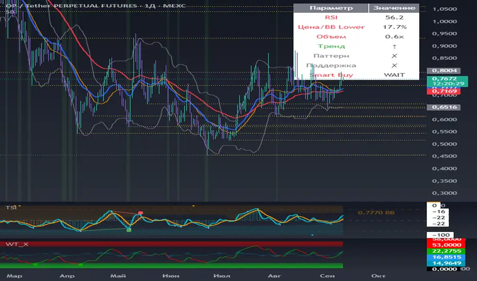
Smart Buyer by [Imagine Income]Smart Buyer Indicator
The "Smart Buyer" indicator identifies optimal entry points for long positions by analyzing the behavior patterns of institutional investors and smart money. This indicator helps traders find the best buying opportunities when professional traders typically accumulate positions.
Key Criteria
The indicator combines multiple technical analysis factors to identify smart buying opportunities:
RSI Oversold Conditions
Detects oversold levels (but not extreme) to avoid catching falling knives
Filters out panic selling while identifying genuine buying opportunities
Price Near Lower Bollinger Band
Identifies when price is trading near the lower Bollinger Band
Ensures buying at the best possible prices within the current range
Increased Volume
Confirms buyer interest through above-average volume
Validates the legitimacy of the potential reversal
Uptrend Confirmation
Only triggers buy signals in an overall upward trend
Ensures alignment with the dominant market direction using EMA crossovers
Reversal Candlestick Patterns
Detects hammer and doji formations
Identifies potential reversal points at key support levels
Proximity to Support Levels
Analyzes pivot lows to identify technical support zones
Increases probability of successful entries near established support
Signal Types
🟢 SB (Smart Buy)
Standard smart buyer signal when multiple criteria align
Indicates a good entry opportunity for long positions
🟢 SB+ (Strong Buy)
Enhanced signal with all criteria met plus low volatility
Represents the highest probability entry points
Visual Elements
Green Background Zone
Highlights optimal buying areas
Shows price ranges where smart money typically accumulates
Yellow Dotted Lines
Mark key support levels based on pivot analysis
Help identify areas where price is likely to find buying interest
Information Table
Real-time display of all indicator parameters
Shows current status of RSI, volume, trend, and other factors
Color-coded for quick assessment (green = bullish, red = bearish)
Settings & Customization
Fully Customizable Parameters
RSI period and oversold levels
Bollinger Bands settings (period and multiplier)
EMA periods for trend analysis
Volume threshold multipliers
Pivot analysis periods
Alert System
Built-in alerts for both standard and strong buy signals
Customizable alert messages for different signal types
Display Options
Toggle signals, zones, and support levels independently
Adapt the indicator appearance to your charting preferences
Optimal Usage
Best Timeframe: Daily
Designed primarily for daily timeframe analysis
Filters out short-term noise while capturing meaningful reversals
Market Application
Works best in trending markets with periodic pullbacks
Ideal for swing trading and position building strategies
Helps identify accumulation zones used by institutional investors
Trading Logic
This indicator replicates the behavior of smart money by:
Buying pullbacks in uptrending markets rather than chasing momentum
Using limit orders at technical support levels
Confirming entries with volume and momentum indicators
Avoiding panic selling by filtering extreme oversold conditions
The Smart Buyer indicator helps retail traders think and act like institutional investors, focusing on high-probability setups where risk-reward ratios are most favorable.
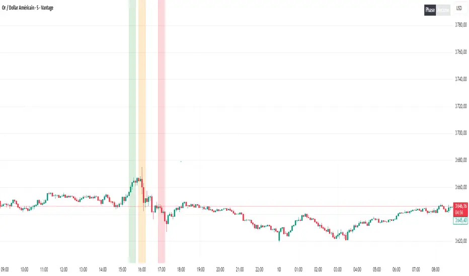
Phase Accumulate/Manipulate/Distribute - NY [nainoa_invest]This TradingView script allows you to identify and visualize the different phases of an asset in the New York market (EST/GMT-4): Accumulation, Manipulation, and Distribution.
Key Features:
Phase Visualization on Chart: Each phase is displayed as a colored rectangle (green for accumulation, orange for manipulation, red for distribution) to easily track market movements.
Dynamic Dashboard: A table shows the current phase in real-time directly on the chart, with customizable colors.
Customizable Settings: You can adjust phase colors, dashboard position and size, and border style.
Precise Time Windows: Phases are automatically calculated based on specific NY session hours for better market behavior tracking.
This script is ideal for traders who want to quickly identify key market phases and make more informed trading decisions.
If you want to use this script, you can contact me directly.
Universal Ratio Trend Matrix [InvestorUnknown]The Universal Ratio Trend Matrix is designed for trend analysis on asset/asset ratios, supporting up to 40 different assets. Its primary purpose is to help identify which assets are outperforming others within a selection, providing a broad overview of market trends through a matrix of ratios. The indicator automatically expands the matrix based on the number of assets chosen, simplifying the process of comparing multiple assets in terms of performance.
Key features include the ability to choose from a narrow selection of indicators to perform the ratio trend analysis, allowing users to apply well-defined metrics to their comparison.
Drawback: Due to the computational intensity involved in calculating ratios across many assets, the indicator has a limitation related to loading speed. TradingView has time limits for calculations, and for users on the basic (free) plan, this could result in frequent errors due to exceeded time limits. To use the indicator effectively, users with any paid plans should run it on timeframes higher than 8h (the lowest timeframe on which it managed to load with 40 assets), as lower timeframes may not reliably load.
Indicators:
RSI_raw: Simple function to calculate the Relative Strength Index (RSI) of a source (asset price).
RSI_sma: Calculates RSI followed by a Simple Moving Average (SMA).
RSI_ema: Calculates RSI followed by an Exponential Moving Average (EMA).
CCI: Calculates the Commodity Channel Index (CCI).
Fisher: Implements the Fisher Transform to normalize prices.
Utility Functions:
f_remove_exchange_name: Strips the exchange name from asset tickers (e.g., "INDEX:BTCUSD" to "BTCUSD").
f_remove_exchange_name(simple string name) =>
string parts = str.split(name, ":")
string result = array.size(parts) > 1 ? array.get(parts, 1) : name
result
f_get_price: Retrieves the closing price of a given asset ticker using request.security().
f_constant_src: Checks if the source data is constant by comparing multiple consecutive values.
Inputs:
General settings allow users to select the number of tickers for analysis (used_assets) and choose the trend indicator (RSI, CCI, Fisher, etc.).
Table settings customize how trend scores are displayed in terms of text size, header visibility, highlighting options, and top-performing asset identification.
The script includes inputs for up to 40 assets, allowing the user to select various cryptocurrencies (e.g., BTCUSD, ETHUSD, SOLUSD) or other assets for trend analysis.
Price Arrays:
Price values for each asset are stored in variables (price_a1 to price_a40) initialized as na. These prices are updated only for the number of assets specified by the user (used_assets).
Trend scores for each asset are stored in separate arrays
// declare price variables as "na"
var float price_a1 = na, var float price_a2 = na, var float price_a3 = na, var float price_a4 = na, var float price_a5 = na
var float price_a6 = na, var float price_a7 = na, var float price_a8 = na, var float price_a9 = na, var float price_a10 = na
var float price_a11 = na, var float price_a12 = na, var float price_a13 = na, var float price_a14 = na, var float price_a15 = na
var float price_a16 = na, var float price_a17 = na, var float price_a18 = na, var float price_a19 = na, var float price_a20 = na
var float price_a21 = na, var float price_a22 = na, var float price_a23 = na, var float price_a24 = na, var float price_a25 = na
var float price_a26 = na, var float price_a27 = na, var float price_a28 = na, var float price_a29 = na, var float price_a30 = na
var float price_a31 = na, var float price_a32 = na, var float price_a33 = na, var float price_a34 = na, var float price_a35 = na
var float price_a36 = na, var float price_a37 = na, var float price_a38 = na, var float price_a39 = na, var float price_a40 = na
// create "empty" arrays to store trend scores
var a1_array = array.new_int(40, 0), var a2_array = array.new_int(40, 0), var a3_array = array.new_int(40, 0), var a4_array = array.new_int(40, 0)
var a5_array = array.new_int(40, 0), var a6_array = array.new_int(40, 0), var a7_array = array.new_int(40, 0), var a8_array = array.new_int(40, 0)
var a9_array = array.new_int(40, 0), var a10_array = array.new_int(40, 0), var a11_array = array.new_int(40, 0), var a12_array = array.new_int(40, 0)
var a13_array = array.new_int(40, 0), var a14_array = array.new_int(40, 0), var a15_array = array.new_int(40, 0), var a16_array = array.new_int(40, 0)
var a17_array = array.new_int(40, 0), var a18_array = array.new_int(40, 0), var a19_array = array.new_int(40, 0), var a20_array = array.new_int(40, 0)
var a21_array = array.new_int(40, 0), var a22_array = array.new_int(40, 0), var a23_array = array.new_int(40, 0), var a24_array = array.new_int(40, 0)
var a25_array = array.new_int(40, 0), var a26_array = array.new_int(40, 0), var a27_array = array.new_int(40, 0), var a28_array = array.new_int(40, 0)
var a29_array = array.new_int(40, 0), var a30_array = array.new_int(40, 0), var a31_array = array.new_int(40, 0), var a32_array = array.new_int(40, 0)
var a33_array = array.new_int(40, 0), var a34_array = array.new_int(40, 0), var a35_array = array.new_int(40, 0), var a36_array = array.new_int(40, 0)
var a37_array = array.new_int(40, 0), var a38_array = array.new_int(40, 0), var a39_array = array.new_int(40, 0), var a40_array = array.new_int(40, 0)
f_get_price(simple string ticker) =>
request.security(ticker, "", close)
// Prices for each USED asset
f_get_asset_price(asset_number, ticker) =>
if (used_assets >= asset_number)
f_get_price(ticker)
else
na
// overwrite empty variables with the prices if "used_assets" is greater or equal to the asset number
if barstate.isconfirmed // use barstate.isconfirmed to avoid "na prices" and calculation errors that result in empty cells in the table
price_a1 := f_get_asset_price(1, asset1), price_a2 := f_get_asset_price(2, asset2), price_a3 := f_get_asset_price(3, asset3), price_a4 := f_get_asset_price(4, asset4)
price_a5 := f_get_asset_price(5, asset5), price_a6 := f_get_asset_price(6, asset6), price_a7 := f_get_asset_price(7, asset7), price_a8 := f_get_asset_price(8, asset8)
price_a9 := f_get_asset_price(9, asset9), price_a10 := f_get_asset_price(10, asset10), price_a11 := f_get_asset_price(11, asset11), price_a12 := f_get_asset_price(12, asset12)
price_a13 := f_get_asset_price(13, asset13), price_a14 := f_get_asset_price(14, asset14), price_a15 := f_get_asset_price(15, asset15), price_a16 := f_get_asset_price(16, asset16)
price_a17 := f_get_asset_price(17, asset17), price_a18 := f_get_asset_price(18, asset18), price_a19 := f_get_asset_price(19, asset19), price_a20 := f_get_asset_price(20, asset20)
price_a21 := f_get_asset_price(21, asset21), price_a22 := f_get_asset_price(22, asset22), price_a23 := f_get_asset_price(23, asset23), price_a24 := f_get_asset_price(24, asset24)
price_a25 := f_get_asset_price(25, asset25), price_a26 := f_get_asset_price(26, asset26), price_a27 := f_get_asset_price(27, asset27), price_a28 := f_get_asset_price(28, asset28)
price_a29 := f_get_asset_price(29, asset29), price_a30 := f_get_asset_price(30, asset30), price_a31 := f_get_asset_price(31, asset31), price_a32 := f_get_asset_price(32, asset32)
price_a33 := f_get_asset_price(33, asset33), price_a34 := f_get_asset_price(34, asset34), price_a35 := f_get_asset_price(35, asset35), price_a36 := f_get_asset_price(36, asset36)
price_a37 := f_get_asset_price(37, asset37), price_a38 := f_get_asset_price(38, asset38), price_a39 := f_get_asset_price(39, asset39), price_a40 := f_get_asset_price(40, asset40)
Universal Indicator Calculation (f_calc_score):
This function allows switching between different trend indicators (RSI, CCI, Fisher) for flexibility.
It uses a switch-case structure to calculate the indicator score, where a positive trend is denoted by 1 and a negative trend by 0. Each indicator has its own logic to determine whether the asset is trending up or down.
// use switch to allow "universality" in indicator selection
f_calc_score(source, trend_indicator, int_1, int_2) =>
int score = na
if (not f_constant_src(source)) and source > 0.0 // Skip if you are using the same assets for ratio (for example BTC/BTC)
x = switch trend_indicator
"RSI (Raw)" => RSI_raw(source, int_1)
"RSI (SMA)" => RSI_sma(source, int_1, int_2)
"RSI (EMA)" => RSI_ema(source, int_1, int_2)
"CCI" => CCI(source, int_1)
"Fisher" => Fisher(source, int_1)
y = switch trend_indicator
"RSI (Raw)" => x > 50 ? 1 : 0
"RSI (SMA)" => x > 50 ? 1 : 0
"RSI (EMA)" => x > 50 ? 1 : 0
"CCI" => x > 0 ? 1 : 0
"Fisher" => x > x ? 1 : 0
score := y
else
score := 0
score
Array Setting Function (f_array_set):
This function populates an array with scores calculated for each asset based on a base price (p_base) divided by the prices of the individual assets.
It processes multiple assets (up to 40), calling the f_calc_score function for each.
// function to set values into the arrays
f_array_set(a_array, p_base) =>
array.set(a_array, 0, f_calc_score(p_base / price_a1, trend_indicator, int_1, int_2))
array.set(a_array, 1, f_calc_score(p_base / price_a2, trend_indicator, int_1, int_2))
array.set(a_array, 2, f_calc_score(p_base / price_a3, trend_indicator, int_1, int_2))
array.set(a_array, 3, f_calc_score(p_base / price_a4, trend_indicator, int_1, int_2))
array.set(a_array, 4, f_calc_score(p_base / price_a5, trend_indicator, int_1, int_2))
array.set(a_array, 5, f_calc_score(p_base / price_a6, trend_indicator, int_1, int_2))
array.set(a_array, 6, f_calc_score(p_base / price_a7, trend_indicator, int_1, int_2))
array.set(a_array, 7, f_calc_score(p_base / price_a8, trend_indicator, int_1, int_2))
array.set(a_array, 8, f_calc_score(p_base / price_a9, trend_indicator, int_1, int_2))
array.set(a_array, 9, f_calc_score(p_base / price_a10, trend_indicator, int_1, int_2))
array.set(a_array, 10, f_calc_score(p_base / price_a11, trend_indicator, int_1, int_2))
array.set(a_array, 11, f_calc_score(p_base / price_a12, trend_indicator, int_1, int_2))
array.set(a_array, 12, f_calc_score(p_base / price_a13, trend_indicator, int_1, int_2))
array.set(a_array, 13, f_calc_score(p_base / price_a14, trend_indicator, int_1, int_2))
array.set(a_array, 14, f_calc_score(p_base / price_a15, trend_indicator, int_1, int_2))
array.set(a_array, 15, f_calc_score(p_base / price_a16, trend_indicator, int_1, int_2))
array.set(a_array, 16, f_calc_score(p_base / price_a17, trend_indicator, int_1, int_2))
array.set(a_array, 17, f_calc_score(p_base / price_a18, trend_indicator, int_1, int_2))
array.set(a_array, 18, f_calc_score(p_base / price_a19, trend_indicator, int_1, int_2))
array.set(a_array, 19, f_calc_score(p_base / price_a20, trend_indicator, int_1, int_2))
array.set(a_array, 20, f_calc_score(p_base / price_a21, trend_indicator, int_1, int_2))
array.set(a_array, 21, f_calc_score(p_base / price_a22, trend_indicator, int_1, int_2))
array.set(a_array, 22, f_calc_score(p_base / price_a23, trend_indicator, int_1, int_2))
array.set(a_array, 23, f_calc_score(p_base / price_a24, trend_indicator, int_1, int_2))
array.set(a_array, 24, f_calc_score(p_base / price_a25, trend_indicator, int_1, int_2))
array.set(a_array, 25, f_calc_score(p_base / price_a26, trend_indicator, int_1, int_2))
array.set(a_array, 26, f_calc_score(p_base / price_a27, trend_indicator, int_1, int_2))
array.set(a_array, 27, f_calc_score(p_base / price_a28, trend_indicator, int_1, int_2))
array.set(a_array, 28, f_calc_score(p_base / price_a29, trend_indicator, int_1, int_2))
array.set(a_array, 29, f_calc_score(p_base / price_a30, trend_indicator, int_1, int_2))
array.set(a_array, 30, f_calc_score(p_base / price_a31, trend_indicator, int_1, int_2))
array.set(a_array, 31, f_calc_score(p_base / price_a32, trend_indicator, int_1, int_2))
array.set(a_array, 32, f_calc_score(p_base / price_a33, trend_indicator, int_1, int_2))
array.set(a_array, 33, f_calc_score(p_base / price_a34, trend_indicator, int_1, int_2))
array.set(a_array, 34, f_calc_score(p_base / price_a35, trend_indicator, int_1, int_2))
array.set(a_array, 35, f_calc_score(p_base / price_a36, trend_indicator, int_1, int_2))
array.set(a_array, 36, f_calc_score(p_base / price_a37, trend_indicator, int_1, int_2))
array.set(a_array, 37, f_calc_score(p_base / price_a38, trend_indicator, int_1, int_2))
array.set(a_array, 38, f_calc_score(p_base / price_a39, trend_indicator, int_1, int_2))
array.set(a_array, 39, f_calc_score(p_base / price_a40, trend_indicator, int_1, int_2))
a_array
Conditional Array Setting (f_arrayset):
This function checks if the number of used assets is greater than or equal to a specified number before populating the arrays.
// only set values into arrays for USED assets
f_arrayset(asset_number, a_array, p_base) =>
if (used_assets >= asset_number)
f_array_set(a_array, p_base)
else
na
Main Logic
The main logic initializes arrays to store scores for each asset. Each array corresponds to one asset's performance score.
Setting Trend Values: The code calls f_arrayset for each asset, populating the respective arrays with calculated scores based on the asset prices.
Combining Arrays: A combined_array is created to hold all the scores from individual asset arrays. This array facilitates further analysis, allowing for an overview of the performance scores of all assets at once.
// create a combined array (work-around since pinescript doesn't support having array of arrays)
var combined_array = array.new_int(40 * 40, 0)
if barstate.islast
for i = 0 to 39
array.set(combined_array, i, array.get(a1_array, i))
array.set(combined_array, i + (40 * 1), array.get(a2_array, i))
array.set(combined_array, i + (40 * 2), array.get(a3_array, i))
array.set(combined_array, i + (40 * 3), array.get(a4_array, i))
array.set(combined_array, i + (40 * 4), array.get(a5_array, i))
array.set(combined_array, i + (40 * 5), array.get(a6_array, i))
array.set(combined_array, i + (40 * 6), array.get(a7_array, i))
array.set(combined_array, i + (40 * 7), array.get(a8_array, i))
array.set(combined_array, i + (40 * 8), array.get(a9_array, i))
array.set(combined_array, i + (40 * 9), array.get(a10_array, i))
array.set(combined_array, i + (40 * 10), array.get(a11_array, i))
array.set(combined_array, i + (40 * 11), array.get(a12_array, i))
array.set(combined_array, i + (40 * 12), array.get(a13_array, i))
array.set(combined_array, i + (40 * 13), array.get(a14_array, i))
array.set(combined_array, i + (40 * 14), array.get(a15_array, i))
array.set(combined_array, i + (40 * 15), array.get(a16_array, i))
array.set(combined_array, i + (40 * 16), array.get(a17_array, i))
array.set(combined_array, i + (40 * 17), array.get(a18_array, i))
array.set(combined_array, i + (40 * 18), array.get(a19_array, i))
array.set(combined_array, i + (40 * 19), array.get(a20_array, i))
array.set(combined_array, i + (40 * 20), array.get(a21_array, i))
array.set(combined_array, i + (40 * 21), array.get(a22_array, i))
array.set(combined_array, i + (40 * 22), array.get(a23_array, i))
array.set(combined_array, i + (40 * 23), array.get(a24_array, i))
array.set(combined_array, i + (40 * 24), array.get(a25_array, i))
array.set(combined_array, i + (40 * 25), array.get(a26_array, i))
array.set(combined_array, i + (40 * 26), array.get(a27_array, i))
array.set(combined_array, i + (40 * 27), array.get(a28_array, i))
array.set(combined_array, i + (40 * 28), array.get(a29_array, i))
array.set(combined_array, i + (40 * 29), array.get(a30_array, i))
array.set(combined_array, i + (40 * 30), array.get(a31_array, i))
array.set(combined_array, i + (40 * 31), array.get(a32_array, i))
array.set(combined_array, i + (40 * 32), array.get(a33_array, i))
array.set(combined_array, i + (40 * 33), array.get(a34_array, i))
array.set(combined_array, i + (40 * 34), array.get(a35_array, i))
array.set(combined_array, i + (40 * 35), array.get(a36_array, i))
array.set(combined_array, i + (40 * 36), array.get(a37_array, i))
array.set(combined_array, i + (40 * 37), array.get(a38_array, i))
array.set(combined_array, i + (40 * 38), array.get(a39_array, i))
array.set(combined_array, i + (40 * 39), array.get(a40_array, i))
Calculating Sums: A separate array_sums is created to store the total score for each asset by summing the values of their respective score arrays. This allows for easy comparison of overall performance.
Ranking Assets: The final part of the code ranks the assets based on their total scores stored in array_sums. It assigns a rank to each asset, where the asset with the highest score receives the highest rank.
// create array for asset RANK based on array.sum
var ranks = array.new_int(used_assets, 0)
// for loop that calculates the rank of each asset
if barstate.islast
for i = 0 to (used_assets - 1)
int rank = 1
for x = 0 to (used_assets - 1)
if i != x
if array.get(array_sums, i) < array.get(array_sums, x)
rank := rank + 1
array.set(ranks, i, rank)
Dynamic Table Creation
Initialization: The table is initialized with a base structure that includes headers for asset names, scores, and ranks. The headers are set to remain constant, ensuring clarity for users as they interpret the displayed data.
Data Population: As scores are calculated for each asset, the corresponding values are dynamically inserted into the table. This is achieved through a loop that iterates over the scores and ranks stored in the combined_array and array_sums, respectively.
Automatic Extending Mechanism
Variable Asset Count: The code checks the number of assets defined by the user. Instead of hardcoding the number of rows in the table, it uses a variable to determine the extent of the data that needs to be displayed. This allows the table to expand or contract based on the number of assets being analyzed.
Dynamic Row Generation: Within the loop that populates the table, the code appends new rows for each asset based on the current asset count. The structure of each row includes the asset name, its score, and its rank, ensuring that the table remains consistent regardless of how many assets are involved.
// Automatically extending table based on the number of used assets
var table table = table.new(position.bottom_center, 50, 50, color.new(color.black, 100), color.white, 3, color.white, 1)
if barstate.islast
if not hide_head
table.cell(table, 0, 0, "Universal Ratio Trend Matrix", text_color = color.white, bgcolor = #010c3b, text_size = fontSize)
table.merge_cells(table, 0, 0, used_assets + 3, 0)
if not hide_inps
table.cell(table, 0, 1,
text = "Inputs: You are using " + str.tostring(trend_indicator) + ", which takes: " + str.tostring(f_get_input(trend_indicator)),
text_color = color.white, text_size = fontSize), table.merge_cells(table, 0, 1, used_assets + 3, 1)
table.cell(table, 0, 2, "Assets", text_color = color.white, text_size = fontSize, bgcolor = #010c3b)
for x = 0 to (used_assets - 1)
table.cell(table, x + 1, 2, text = str.tostring(array.get(assets, x)), text_color = color.white, bgcolor = #010c3b, text_size = fontSize)
table.cell(table, 0, x + 3, text = str.tostring(array.get(assets, x)), text_color = color.white, bgcolor = f_asset_col(array.get(ranks, x)), text_size = fontSize)
for r = 0 to (used_assets - 1)
for c = 0 to (used_assets - 1)
table.cell(table, c + 1, r + 3, text = str.tostring(array.get(combined_array, c + (r * 40))),
text_color = hl_type == "Text" ? f_get_col(array.get(combined_array, c + (r * 40))) : color.white, text_size = fontSize,
bgcolor = hl_type == "Background" ? f_get_col(array.get(combined_array, c + (r * 40))) : na)
for x = 0 to (used_assets - 1)
table.cell(table, x + 1, x + 3, "", bgcolor = #010c3b)
table.cell(table, used_assets + 1, 2, "", bgcolor = #010c3b)
for x = 0 to (used_assets - 1)
table.cell(table, used_assets + 1, x + 3, "==>", text_color = color.white)
table.cell(table, used_assets + 2, 2, "SUM", text_color = color.white, text_size = fontSize, bgcolor = #010c3b)
table.cell(table, used_assets + 3, 2, "RANK", text_color = color.white, text_size = fontSize, bgcolor = #010c3b)
for x = 0 to (used_assets - 1)
table.cell(table, used_assets + 2, x + 3,
text = str.tostring(array.get(array_sums, x)),
text_color = color.white, text_size = fontSize,
bgcolor = f_highlight_sum(array.get(array_sums, x), array.get(ranks, x)))
table.cell(table, used_assets + 3, x + 3,
text = str.tostring(array.get(ranks, x)),
text_color = color.white, text_size = fontSize,
bgcolor = f_highlight_rank(array.get(ranks, x)))

Markov Chain [3D] | FractalystWhat exactly is a Markov Chain?
This indicator uses a Markov Chain model to analyze, quantify, and visualize the transitions between market regimes (Bull, Bear, Neutral) on your chart. It dynamically detects these regimes in real-time, calculates transition probabilities, and displays them as animated 3D spheres and arrows, giving traders intuitive insight into current and future market conditions.
How does a Markov Chain work, and how should I read this spheres-and-arrows diagram?
Think of three weather modes: Sunny, Rainy, Cloudy.
Each sphere is one mode. The loop on a sphere means “stay the same next step” (e.g., Sunny again tomorrow).
The arrows leaving a sphere show where things usually go next if they change (e.g., Sunny moving to Cloudy).
Some paths matter more than others. A more prominent loop means the current mode tends to persist. A more prominent outgoing arrow means a change to that destination is the usual next step.
Direction isn’t symmetric: moving Sunny→Cloudy can behave differently than Cloudy→Sunny.
Now relabel the spheres to markets: Bull, Bear, Neutral.
Spheres: market regimes (uptrend, downtrend, range).
Self‑loop: tendency for the current regime to continue on the next bar.
Arrows: the most common next regime if a switch happens.
How to read: Start at the sphere that matches current bar state. If the loop stands out, expect continuation. If one outgoing path stands out, that switch is the typical next step. Opposite directions can differ (Bear→Neutral doesn’t have to match Neutral→Bear).
What states and transitions are shown?
The three market states visualized are:
Bullish (Bull): Upward or strong-market regime.
Bearish (Bear): Downward or weak-market regime.
Neutral: Sideways or range-bound regime.
Bidirectional animated arrows and probability labels show how likely the market is to move from one regime to another (e.g., Bull → Bear or Neutral → Bull).
How does the regime detection system work?
You can use either built-in price returns (based on adaptive Z-score normalization) or supply three custom indicators (such as volume, oscillators, etc.).
Values are statistically normalized (Z-scored) over a configurable lookback period.
The normalized outputs are classified into Bull, Bear, or Neutral zones.
If using three indicators, their regime signals are averaged and smoothed for robustness.
How are transition probabilities calculated?
On every confirmed bar, the algorithm tracks the sequence of detected market states, then builds a rolling window of transitions.
The code maintains a transition count matrix for all regime pairs (e.g., Bull → Bear).
Transition probabilities are extracted for each possible state change using Laplace smoothing for numerical stability, and frequently updated in real-time.
What is unique about the visualization?
3D animated spheres represent each regime and change visually when active.
Animated, bidirectional arrows reveal transition probabilities and allow you to see both dominant and less likely regime flows.
Particles (moving dots) animate along the arrows, enhancing the perception of regime flow direction and speed.
All elements dynamically update with each new price bar, providing a live market map in an intuitive, engaging format.
Can I use custom indicators for regime classification?
Yes! Enable the "Custom Indicators" switch and select any three chart series as inputs. These will be normalized and combined (each with equal weight), broadening the regime classification beyond just price-based movement.
What does the “Lookback Period” control?
Lookback Period (default: 100) sets how much historical data builds the probability matrix. Shorter periods adapt faster to regime changes but may be noisier. Longer periods are more stable but slower to adapt.
How is this different from a Hidden Markov Model (HMM)?
It sets the window for both regime detection and probability calculations. Lower values make the system more reactive, but potentially noisier. Higher values smooth estimates and make the system more robust.
How is this Markov Chain different from a Hidden Markov Model (HMM)?
Markov Chain (as here): All market regimes (Bull, Bear, Neutral) are directly observable on the chart. The transition matrix is built from actual detected regimes, keeping the model simple and interpretable.
Hidden Markov Model: The actual regimes are unobservable ("hidden") and must be inferred from market output or indicator "emissions" using statistical learning algorithms. HMMs are more complex, can capture more subtle structure, but are harder to visualize and require additional machine learning steps for training.
A standard Markov Chain models transitions between observable states using a simple transition matrix, while a Hidden Markov Model assumes the true states are hidden (latent) and must be inferred from observable “emissions” like price or volume data. In practical terms, a Markov Chain is transparent and easier to implement and interpret; an HMM is more expressive but requires statistical inference to estimate hidden states from data.
Markov Chain: states are observable; you directly count or estimate transition probabilities between visible states. This makes it simpler, faster, and easier to validate and tune.
HMM: states are hidden; you only observe emissions generated by those latent states. Learning involves machine learning/statistical algorithms (commonly Baum–Welch/EM for training and Viterbi for decoding) to infer both the transition dynamics and the most likely hidden state sequence from data.
How does the indicator avoid “repainting” or look-ahead bias?
All regime changes and matrix updates happen only on confirmed (closed) bars, so no future data is leaked, ensuring reliable real-time operation.
Are there practical tuning tips?
Tune the Lookback Period for your asset/timeframe: shorter for fast markets, longer for stability.
Use custom indicators if your asset has unique regime drivers.
Watch for rapid changes in transition probabilities as early warning of a possible regime shift.
Who is this indicator for?
Quants and quantitative researchers exploring probabilistic market modeling, especially those interested in regime-switching dynamics and Markov models.
Programmers and system developers who need a probabilistic regime filter for systematic and algorithmic backtesting:
The Markov Chain indicator is ideally suited for programmatic integration via its bias output (1 = Bull, 0 = Neutral, -1 = Bear).
Although the visualization is engaging, the core output is designed for automated, rules-based workflows—not for discretionary/manual trading decisions.
Developers can connect the indicator’s output directly to their Pine Script logic (using input.source()), allowing rapid and robust backtesting of regime-based strategies.
It acts as a plug-and-play regime filter: simply plug the bias output into your entry/exit logic, and you have a scientifically robust, probabilistically-derived signal for filtering, timing, position sizing, or risk regimes.
The MC's output is intentionally "trinary" (1/0/-1), focusing on clear regime states for unambiguous decision-making in code. If you require nuanced, multi-probability or soft-label state vectors, consider expanding the indicator or stacking it with a probability-weighted logic layer in your scripting.
Because it avoids subjectivity, this approach is optimal for systematic quants, algo developers building backtested, repeatable strategies based on probabilistic regime analysis.
What's the mathematical foundation behind this?
The mathematical foundation behind this Markov Chain indicator—and probabilistic regime detection in finance—draws from two principal models: the (standard) Markov Chain and the Hidden Markov Model (HMM).
How to use this indicator programmatically?
The Markov Chain indicator automatically exports a bias value (+1 for Bullish, -1 for Bearish, 0 for Neutral) as a plot visible in the Data Window. This allows you to integrate its regime signal into your own scripts and strategies for backtesting, automation, or live trading.
Step-by-Step Integration with Pine Script (input.source)
Add the Markov Chain indicator to your chart.
This must be done first, since your custom script will "pull" the bias signal from the indicator's plot.
In your strategy, create an input using input.source()
Example:
//@version=5
strategy("MC Bias Strategy Example")
mcBias = input.source(close, "MC Bias Source")
After saving, go to your script’s settings. For the “MC Bias Source” input, select the plot/output of the Markov Chain indicator (typically its bias plot).
Use the bias in your trading logic
Example (long only on Bull, flat otherwise):
if mcBias == 1
strategy.entry("Long", strategy.long)
else
strategy.close("Long")
For more advanced workflows, combine mcBias with additional filters or trailing stops.
How does this work behind-the-scenes?
TradingView’s input.source() lets you use any plot from another indicator as a real-time, “live” data feed in your own script (source).
The selected bias signal is available to your Pine code as a variable, enabling logical decisions based on regime (trend-following, mean-reversion, etc.).
This enables powerful strategy modularity : decouple regime detection from entry/exit logic, allowing fast experimentation without rewriting core signal code.
Integrating 45+ Indicators with Your Markov Chain — How & Why
The Enhanced Custom Indicators Export script exports a massive suite of over 45 technical indicators—ranging from classic momentum (RSI, MACD, Stochastic, etc.) to trend, volume, volatility, and oscillator tools—all pre-calculated, centered/scaled, and available as plots.
// Enhanced Custom Indicators Export - 45 Technical Indicators
// Comprehensive technical analysis suite for advanced market regime detection
//@version=6
indicator('Enhanced Custom Indicators Export | Fractalyst', shorttitle='Enhanced CI Export', overlay=false, scale=scale.right, max_labels_count=500, max_lines_count=500)
// |----- Input Parameters -----| //
momentum_group = "Momentum Indicators"
trend_group = "Trend Indicators"
volume_group = "Volume Indicators"
volatility_group = "Volatility Indicators"
oscillator_group = "Oscillator Indicators"
display_group = "Display Settings"
// Common lengths
length_14 = input.int(14, "Standard Length (14)", minval=1, maxval=100, group=momentum_group)
length_20 = input.int(20, "Medium Length (20)", minval=1, maxval=200, group=trend_group)
length_50 = input.int(50, "Long Length (50)", minval=1, maxval=200, group=trend_group)
// Display options
show_table = input.bool(true, "Show Values Table", group=display_group)
table_size = input.string("Small", "Table Size", options= , group=display_group)
// |----- MOMENTUM INDICATORS (15 indicators) -----| //
// 1. RSI (Relative Strength Index)
rsi_14 = ta.rsi(close, length_14)
rsi_centered = rsi_14 - 50
// 2. Stochastic Oscillator
stoch_k = ta.stoch(close, high, low, length_14)
stoch_d = ta.sma(stoch_k, 3)
stoch_centered = stoch_k - 50
// 3. Williams %R
williams_r = ta.stoch(close, high, low, length_14) - 100
// 4. MACD (Moving Average Convergence Divergence)
= ta.macd(close, 12, 26, 9)
// 5. Momentum (Rate of Change)
momentum = ta.mom(close, length_14)
momentum_pct = (momentum / close ) * 100
// 6. Rate of Change (ROC)
roc = ta.roc(close, length_14)
// 7. Commodity Channel Index (CCI)
cci = ta.cci(close, length_20)
// 8. Money Flow Index (MFI)
mfi = ta.mfi(close, length_14)
mfi_centered = mfi - 50
// 9. Awesome Oscillator (AO)
ao = ta.sma(hl2, 5) - ta.sma(hl2, 34)
// 10. Accelerator Oscillator (AC)
ac = ao - ta.sma(ao, 5)
// 11. Chande Momentum Oscillator (CMO)
cmo = ta.cmo(close, length_14)
// 12. Detrended Price Oscillator (DPO)
dpo = close - ta.sma(close, length_20)
// 13. Price Oscillator (PPO)
ppo = ta.sma(close, 12) - ta.sma(close, 26)
ppo_pct = (ppo / ta.sma(close, 26)) * 100
// 14. TRIX
trix_ema1 = ta.ema(close, length_14)
trix_ema2 = ta.ema(trix_ema1, length_14)
trix_ema3 = ta.ema(trix_ema2, length_14)
trix = ta.roc(trix_ema3, 1) * 10000
// 15. Klinger Oscillator
klinger = ta.ema(volume * (high + low + close) / 3, 34) - ta.ema(volume * (high + low + close) / 3, 55)
// 16. Fisher Transform
fisher_hl2 = 0.5 * (hl2 - ta.lowest(hl2, 10)) / (ta.highest(hl2, 10) - ta.lowest(hl2, 10)) - 0.25
fisher = 0.5 * math.log((1 + fisher_hl2) / (1 - fisher_hl2))
// 17. Stochastic RSI
stoch_rsi = ta.stoch(rsi_14, rsi_14, rsi_14, length_14)
stoch_rsi_centered = stoch_rsi - 50
// 18. Relative Vigor Index (RVI)
rvi_num = ta.swma(close - open)
rvi_den = ta.swma(high - low)
rvi = rvi_den != 0 ? rvi_num / rvi_den : 0
// 19. Balance of Power (BOP)
bop = (close - open) / (high - low)
// |----- TREND INDICATORS (10 indicators) -----| //
// 20. Simple Moving Average Momentum
sma_20 = ta.sma(close, length_20)
sma_momentum = ((close - sma_20) / sma_20) * 100
// 21. Exponential Moving Average Momentum
ema_20 = ta.ema(close, length_20)
ema_momentum = ((close - ema_20) / ema_20) * 100
// 22. Parabolic SAR
sar = ta.sar(0.02, 0.02, 0.2)
sar_trend = close > sar ? 1 : -1
// 23. Linear Regression Slope
lr_slope = ta.linreg(close, length_20, 0) - ta.linreg(close, length_20, 1)
// 24. Moving Average Convergence (MAC)
mac = ta.sma(close, 10) - ta.sma(close, 30)
// 25. Trend Intensity Index (TII)
tii_sum = 0.0
for i = 1 to length_20
tii_sum += close > close ? 1 : 0
tii = (tii_sum / length_20) * 100
// 26. Ichimoku Cloud Components
ichimoku_tenkan = (ta.highest(high, 9) + ta.lowest(low, 9)) / 2
ichimoku_kijun = (ta.highest(high, 26) + ta.lowest(low, 26)) / 2
ichimoku_signal = ichimoku_tenkan > ichimoku_kijun ? 1 : -1
// 27. MESA Adaptive Moving Average (MAMA)
mama_alpha = 2.0 / (length_20 + 1)
mama = ta.ema(close, length_20)
mama_momentum = ((close - mama) / mama) * 100
// 28. Zero Lag Exponential Moving Average (ZLEMA)
zlema_lag = math.round((length_20 - 1) / 2)
zlema_data = close + (close - close )
zlema = ta.ema(zlema_data, length_20)
zlema_momentum = ((close - zlema) / zlema) * 100
// |----- VOLUME INDICATORS (6 indicators) -----| //
// 29. On-Balance Volume (OBV)
obv = ta.obv
// 30. Volume Rate of Change (VROC)
vroc = ta.roc(volume, length_14)
// 31. Price Volume Trend (PVT)
pvt = ta.pvt
// 32. Negative Volume Index (NVI)
nvi = 0.0
nvi := volume < volume ? nvi + ((close - close ) / close ) * nvi : nvi
// 33. Positive Volume Index (PVI)
pvi = 0.0
pvi := volume > volume ? pvi + ((close - close ) / close ) * pvi : pvi
// 34. Volume Oscillator
vol_osc = ta.sma(volume, 5) - ta.sma(volume, 10)
// 35. Ease of Movement (EOM)
eom_distance = high - low
eom_box_height = volume / 1000000
eom = eom_box_height != 0 ? eom_distance / eom_box_height : 0
eom_sma = ta.sma(eom, length_14)
// 36. Force Index
force_index = volume * (close - close )
force_index_sma = ta.sma(force_index, length_14)
// |----- VOLATILITY INDICATORS (10 indicators) -----| //
// 37. Average True Range (ATR)
atr = ta.atr(length_14)
atr_pct = (atr / close) * 100
// 38. Bollinger Bands Position
bb_basis = ta.sma(close, length_20)
bb_dev = 2.0 * ta.stdev(close, length_20)
bb_upper = bb_basis + bb_dev
bb_lower = bb_basis - bb_dev
bb_position = bb_dev != 0 ? (close - bb_basis) / bb_dev : 0
bb_width = bb_dev != 0 ? (bb_upper - bb_lower) / bb_basis * 100 : 0
// 39. Keltner Channels Position
kc_basis = ta.ema(close, length_20)
kc_range = ta.ema(ta.tr, length_20)
kc_upper = kc_basis + (2.0 * kc_range)
kc_lower = kc_basis - (2.0 * kc_range)
kc_position = kc_range != 0 ? (close - kc_basis) / kc_range : 0
// 40. Donchian Channels Position
dc_upper = ta.highest(high, length_20)
dc_lower = ta.lowest(low, length_20)
dc_basis = (dc_upper + dc_lower) / 2
dc_position = (dc_upper - dc_lower) != 0 ? (close - dc_basis) / (dc_upper - dc_lower) : 0
// 41. Standard Deviation
std_dev = ta.stdev(close, length_20)
std_dev_pct = (std_dev / close) * 100
// 42. Relative Volatility Index (RVI)
rvi_up = ta.stdev(close > close ? close : 0, length_14)
rvi_down = ta.stdev(close < close ? close : 0, length_14)
rvi_total = rvi_up + rvi_down
rvi_volatility = rvi_total != 0 ? (rvi_up / rvi_total) * 100 : 50
// 43. Historical Volatility
hv_returns = math.log(close / close )
hv = ta.stdev(hv_returns, length_20) * math.sqrt(252) * 100
// 44. Garman-Klass Volatility
gk_vol = math.log(high/low) * math.log(high/low) - (2*math.log(2)-1) * math.log(close/open) * math.log(close/open)
gk_volatility = math.sqrt(ta.sma(gk_vol, length_20)) * 100
// 45. Parkinson Volatility
park_vol = math.log(high/low) * math.log(high/low)
parkinson = math.sqrt(ta.sma(park_vol, length_20) / (4 * math.log(2))) * 100
// 46. Rogers-Satchell Volatility
rs_vol = math.log(high/close) * math.log(high/open) + math.log(low/close) * math.log(low/open)
rogers_satchell = math.sqrt(ta.sma(rs_vol, length_20)) * 100
// |----- OSCILLATOR INDICATORS (5 indicators) -----| //
// 47. Elder Ray Index
elder_bull = high - ta.ema(close, 13)
elder_bear = low - ta.ema(close, 13)
elder_power = elder_bull + elder_bear
// 48. Schaff Trend Cycle (STC)
stc_macd = ta.ema(close, 23) - ta.ema(close, 50)
stc_k = ta.stoch(stc_macd, stc_macd, stc_macd, 10)
stc_d = ta.ema(stc_k, 3)
stc = ta.stoch(stc_d, stc_d, stc_d, 10)
// 49. Coppock Curve
coppock_roc1 = ta.roc(close, 14)
coppock_roc2 = ta.roc(close, 11)
coppock = ta.wma(coppock_roc1 + coppock_roc2, 10)
// 50. Know Sure Thing (KST)
kst_roc1 = ta.roc(close, 10)
kst_roc2 = ta.roc(close, 15)
kst_roc3 = ta.roc(close, 20)
kst_roc4 = ta.roc(close, 30)
kst = ta.sma(kst_roc1, 10) + 2*ta.sma(kst_roc2, 10) + 3*ta.sma(kst_roc3, 10) + 4*ta.sma(kst_roc4, 15)
// 51. Percentage Price Oscillator (PPO)
ppo_line = ((ta.ema(close, 12) - ta.ema(close, 26)) / ta.ema(close, 26)) * 100
ppo_signal = ta.ema(ppo_line, 9)
ppo_histogram = ppo_line - ppo_signal
// |----- PLOT MAIN INDICATORS -----| //
// Plot key momentum indicators
plot(rsi_centered, title="01_RSI_Centered", color=color.purple, linewidth=1)
plot(stoch_centered, title="02_Stoch_Centered", color=color.blue, linewidth=1)
plot(williams_r, title="03_Williams_R", color=color.red, linewidth=1)
plot(macd_histogram, title="04_MACD_Histogram", color=color.orange, linewidth=1)
plot(cci, title="05_CCI", color=color.green, linewidth=1)
// Plot trend indicators
plot(sma_momentum, title="06_SMA_Momentum", color=color.navy, linewidth=1)
plot(ema_momentum, title="07_EMA_Momentum", color=color.maroon, linewidth=1)
plot(sar_trend, title="08_SAR_Trend", color=color.teal, linewidth=1)
plot(lr_slope, title="09_LR_Slope", color=color.lime, linewidth=1)
plot(mac, title="10_MAC", color=color.fuchsia, linewidth=1)
// Plot volatility indicators
plot(atr_pct, title="11_ATR_Pct", color=color.yellow, linewidth=1)
plot(bb_position, title="12_BB_Position", color=color.aqua, linewidth=1)
plot(kc_position, title="13_KC_Position", color=color.olive, linewidth=1)
plot(std_dev_pct, title="14_StdDev_Pct", color=color.silver, linewidth=1)
plot(bb_width, title="15_BB_Width", color=color.gray, linewidth=1)
// Plot volume indicators
plot(vroc, title="16_VROC", color=color.blue, linewidth=1)
plot(eom_sma, title="17_EOM", color=color.red, linewidth=1)
plot(vol_osc, title="18_Vol_Osc", color=color.green, linewidth=1)
plot(force_index_sma, title="19_Force_Index", color=color.orange, linewidth=1)
plot(obv, title="20_OBV", color=color.purple, linewidth=1)
// Plot additional oscillators
plot(ao, title="21_Awesome_Osc", color=color.navy, linewidth=1)
plot(cmo, title="22_CMO", color=color.maroon, linewidth=1)
plot(dpo, title="23_DPO", color=color.teal, linewidth=1)
plot(trix, title="24_TRIX", color=color.lime, linewidth=1)
plot(fisher, title="25_Fisher", color=color.fuchsia, linewidth=1)
// Plot more momentum indicators
plot(mfi_centered, title="26_MFI_Centered", color=color.yellow, linewidth=1)
plot(ac, title="27_AC", color=color.aqua, linewidth=1)
plot(ppo_pct, title="28_PPO_Pct", color=color.olive, linewidth=1)
plot(stoch_rsi_centered, title="29_StochRSI_Centered", color=color.silver, linewidth=1)
plot(klinger, title="30_Klinger", color=color.gray, linewidth=1)
// Plot trend continuation
plot(tii, title="31_TII", color=color.blue, linewidth=1)
plot(ichimoku_signal, title="32_Ichimoku_Signal", color=color.red, linewidth=1)
plot(mama_momentum, title="33_MAMA_Momentum", color=color.green, linewidth=1)
plot(zlema_momentum, title="34_ZLEMA_Momentum", color=color.orange, linewidth=1)
plot(bop, title="35_BOP", color=color.purple, linewidth=1)
// Plot volume continuation
plot(nvi, title="36_NVI", color=color.navy, linewidth=1)
plot(pvi, title="37_PVI", color=color.maroon, linewidth=1)
plot(momentum_pct, title="38_Momentum_Pct", color=color.teal, linewidth=1)
plot(roc, title="39_ROC", color=color.lime, linewidth=1)
plot(rvi, title="40_RVI", color=color.fuchsia, linewidth=1)
// Plot volatility continuation
plot(dc_position, title="41_DC_Position", color=color.yellow, linewidth=1)
plot(rvi_volatility, title="42_RVI_Volatility", color=color.aqua, linewidth=1)
plot(hv, title="43_Historical_Vol", color=color.olive, linewidth=1)
plot(gk_volatility, title="44_GK_Volatility", color=color.silver, linewidth=1)
plot(parkinson, title="45_Parkinson_Vol", color=color.gray, linewidth=1)
// Plot final oscillators
plot(rogers_satchell, title="46_RS_Volatility", color=color.blue, linewidth=1)
plot(elder_power, title="47_Elder_Power", color=color.red, linewidth=1)
plot(stc, title="48_STC", color=color.green, linewidth=1)
plot(coppock, title="49_Coppock", color=color.orange, linewidth=1)
plot(kst, title="50_KST", color=color.purple, linewidth=1)
// Plot final indicators
plot(ppo_histogram, title="51_PPO_Histogram", color=color.navy, linewidth=1)
plot(pvt, title="52_PVT", color=color.maroon, linewidth=1)
// |----- Reference Lines -----| //
hline(0, "Zero Line", color=color.gray, linestyle=hline.style_dashed, linewidth=1)
hline(50, "Midline", color=color.gray, linestyle=hline.style_dotted, linewidth=1)
hline(-50, "Lower Midline", color=color.gray, linestyle=hline.style_dotted, linewidth=1)
hline(25, "Upper Threshold", color=color.gray, linestyle=hline.style_dotted, linewidth=1)
hline(-25, "Lower Threshold", color=color.gray, linestyle=hline.style_dotted, linewidth=1)
// |----- Enhanced Information Table -----| //
if show_table and barstate.islast
table_position = position.top_right
table_text_size = table_size == "Tiny" ? size.tiny : table_size == "Small" ? size.small : size.normal
var table info_table = table.new(table_position, 3, 18, bgcolor=color.new(color.white, 85), border_width=1, border_color=color.gray)
// Headers
table.cell(info_table, 0, 0, 'Category', text_color=color.black, text_size=table_text_size, bgcolor=color.new(color.blue, 70))
table.cell(info_table, 1, 0, 'Indicator', text_color=color.black, text_size=table_text_size, bgcolor=color.new(color.blue, 70))
table.cell(info_table, 2, 0, 'Value', text_color=color.black, text_size=table_text_size, bgcolor=color.new(color.blue, 70))
// Key Momentum Indicators
table.cell(info_table, 0, 1, 'MOMENTUM', text_color=color.purple, text_size=table_text_size, bgcolor=color.new(color.purple, 90))
table.cell(info_table, 1, 1, 'RSI Centered', text_color=color.purple, text_size=table_text_size)
table.cell(info_table, 2, 1, str.tostring(rsi_centered, '0.00'), text_color=color.purple, text_size=table_text_size)
table.cell(info_table, 0, 2, '', text_color=color.blue, text_size=table_text_size)
table.cell(info_table, 1, 2, 'Stoch Centered', text_color=color.blue, text_size=table_text_size)
table.cell(info_table, 2, 2, str.tostring(stoch_centered, '0.00'), text_color=color.blue, text_size=table_text_size)
table.cell(info_table, 0, 3, '', text_color=color.red, text_size=table_text_size)
table.cell(info_table, 1, 3, 'Williams %R', text_color=color.red, text_size=table_text_size)
table.cell(info_table, 2, 3, str.tostring(williams_r, '0.00'), text_color=color.red, text_size=table_text_size)
table.cell(info_table, 0, 4, '', text_color=color.orange, text_size=table_text_size)
table.cell(info_table, 1, 4, 'MACD Histogram', text_color=color.orange, text_size=table_text_size)
table.cell(info_table, 2, 4, str.tostring(macd_histogram, '0.000'), text_color=color.orange, text_size=table_text_size)
table.cell(info_table, 0, 5, '', text_color=color.green, text_size=table_text_size)
table.cell(info_table, 1, 5, 'CCI', text_color=color.green, text_size=table_text_size)
table.cell(info_table, 2, 5, str.tostring(cci, '0.00'), text_color=color.green, text_size=table_text_size)
// Key Trend Indicators
table.cell(info_table, 0, 6, 'TREND', text_color=color.navy, text_size=table_text_size, bgcolor=color.new(color.navy, 90))
table.cell(info_table, 1, 6, 'SMA Momentum %', text_color=color.navy, text_size=table_text_size)
table.cell(info_table, 2, 6, str.tostring(sma_momentum, '0.00'), text_color=color.navy, text_size=table_text_size)
table.cell(info_table, 0, 7, '', text_color=color.maroon, text_size=table_text_size)
table.cell(info_table, 1, 7, 'EMA Momentum %', text_color=color.maroon, text_size=table_text_size)
table.cell(info_table, 2, 7, str.tostring(ema_momentum, '0.00'), text_color=color.maroon, text_size=table_text_size)
table.cell(info_table, 0, 8, '', text_color=color.teal, text_size=table_text_size)
table.cell(info_table, 1, 8, 'SAR Trend', text_color=color.teal, text_size=table_text_size)
table.cell(info_table, 2, 8, str.tostring(sar_trend, '0'), text_color=color.teal, text_size=table_text_size)
table.cell(info_table, 0, 9, '', text_color=color.lime, text_size=table_text_size)
table.cell(info_table, 1, 9, 'Linear Regression', text_color=color.lime, text_size=table_text_size)
table.cell(info_table, 2, 9, str.tostring(lr_slope, '0.000'), text_color=color.lime, text_size=table_text_size)
// Key Volatility Indicators
table.cell(info_table, 0, 10, 'VOLATILITY', text_color=color.yellow, text_size=table_text_size, bgcolor=color.new(color.yellow, 90))
table.cell(info_table, 1, 10, 'ATR %', text_color=color.yellow, text_size=table_text_size)
table.cell(info_table, 2, 10, str.tostring(atr_pct, '0.00'), text_color=color.yellow, text_size=table_text_size)
table.cell(info_table, 0, 11, '', text_color=color.aqua, text_size=table_text_size)
table.cell(info_table, 1, 11, 'BB Position', text_color=color.aqua, text_size=table_text_size)
table.cell(info_table, 2, 11, str.tostring(bb_position, '0.00'), text_color=color.aqua, text_size=table_text_size)
table.cell(info_table, 0, 12, '', text_color=color.olive, text_size=table_text_size)
table.cell(info_table, 1, 12, 'KC Position', text_color=color.olive, text_size=table_text_size)
table.cell(info_table, 2, 12, str.tostring(kc_position, '0.00'), text_color=color.olive, text_size=table_text_size)
// Key Volume Indicators
table.cell(info_table, 0, 13, 'VOLUME', text_color=color.blue, text_size=table_text_size, bgcolor=color.new(color.blue, 90))
table.cell(info_table, 1, 13, 'Volume ROC', text_color=color.blue, text_size=table_text_size)
table.cell(info_table, 2, 13, str.tostring(vroc, '0.00'), text_color=color.blue, text_size=table_text_size)
table.cell(info_table, 0, 14, '', text_color=color.red, text_size=table_text_size)
table.cell(info_table, 1, 14, 'EOM', text_color=color.red, text_size=table_text_size)
table.cell(info_table, 2, 14, str.tostring(eom_sma, '0.000'), text_color=color.red, text_size=table_text_size)
// Key Oscillators
table.cell(info_table, 0, 15, 'OSCILLATORS', text_color=color.purple, text_size=table_text_size, bgcolor=color.new(color.purple, 90))
table.cell(info_table, 1, 15, 'Awesome Osc', text_color=color.blue, text_size=table_text_size)
table.cell(info_table, 2, 15, str.tostring(ao, '0.000'), text_color=color.blue, text_size=table_text_size)
table.cell(info_table, 0, 16, '', text_color=color.red, text_size=table_text_size)
table.cell(info_table, 1, 16, 'Fisher Transform', text_color=color.red, text_size=table_text_size)
table.cell(info_table, 2, 16, str.tostring(fisher, '0.000'), text_color=color.red, text_size=table_text_size)
// Summary Statistics
table.cell(info_table, 0, 17, 'SUMMARY', text_color=color.black, text_size=table_text_size, bgcolor=color.new(color.gray, 70))
table.cell(info_table, 1, 17, 'Total Indicators: 52', text_color=color.black, text_size=table_text_size)
regime_color = rsi_centered > 10 ? color.green : rsi_centered < -10 ? color.red : color.gray
regime_text = rsi_centered > 10 ? "BULLISH" : rsi_centered < -10 ? "BEARISH" : "NEUTRAL"
table.cell(info_table, 2, 17, regime_text, text_color=regime_color, text_size=table_text_size)
This makes it the perfect “indicator backbone” for quantitative and systematic traders who want to prototype, combine, and test new regime detection models—especially in combination with the Markov Chain indicator.
How to use this script with the Markov Chain for research and backtesting:
Add the Enhanced Indicator Export to your chart.
Every calculated indicator is available as an individual data stream.
Connect the indicator(s) you want as custom input(s) to the Markov Chain’s “Custom Indicators” option.
In the Markov Chain indicator’s settings, turn ON the custom indicator mode.
For each of the three custom indicator inputs, select the exported plot from the Enhanced Export script—the menu lists all 45+ signals by name.
This creates a powerful, modular regime-detection engine where you can mix-and-match momentum, trend, volume, or custom combinations for advanced filtering.
Backtest regime logic directly.
Once you’ve connected your chosen indicators, the Markov Chain script performs regime detection (Bull/Neutral/Bear) based on your selected features—not just price returns.
The regime detection is robust, automatically normalized (using Z-score), and outputs bias (1, -1, 0) for plug-and-play integration.
Export the regime bias for programmatic use.
As described above, use input.source() in your Pine Script strategy or system and link the bias output.
You can now filter signals, control trade direction/size, or design pairs-trading that respect true, indicator-driven market regimes.
With this framework, you’re not limited to static or simplistic regime filters. You can rigorously define, test, and refine what “market regime” means for your strategies—using the technical features that matter most to you.
Optimize your signal generation by backtesting across a universe of meaningful indicator blends.
Enhance risk management with objective, real-time regime boundaries.
Accelerate your research: iterate quickly, swap indicator components, and see results with minimal code changes.
Automate multi-asset or pairs-trading by integrating regime context directly into strategy logic.
Add both scripts to your chart, connect your preferred features, and start investigating your best regime-based trades—entirely within the TradingView ecosystem.
References & Further Reading
Ang, A., & Bekaert, G. (2002). “Regime Switches in Interest Rates.” Journal of Business & Economic Statistics, 20(2), 163–182.
Hamilton, J. D. (1989). “A New Approach to the Economic Analysis of Nonstationary Time Series and the Business Cycle.” Econometrica, 57(2), 357–384.
Markov, A. A. (1906). "Extension of the Limit Theorems of Probability Theory to a Sum of Variables Connected in a Chain." The Notes of the Imperial Academy of Sciences of St. Petersburg.
Guidolin, M., & Timmermann, A. (2007). “Asset Allocation under Multivariate Regime Switching.” Journal of Economic Dynamics and Control, 31(11), 3503–3544.
Murphy, J. J. (1999). Technical Analysis of the Financial Markets. New York Institute of Finance.
Brock, W., Lakonishok, J., & LeBaron, B. (1992). “Simple Technical Trading Rules and the Stochastic Properties of Stock Returns.” Journal of Finance, 47(5), 1731–1764.
Zucchini, W., MacDonald, I. L., & Langrock, R. (2017). Hidden Markov Models for Time Series: An Introduction Using R (2nd ed.). Chapman and Hall/CRC.
On Quantitative Finance and Markov Models:
Lo, A. W., & Hasanhodzic, J. (2009). The Heretics of Finance: Conversations with Leading Practitioners of Technical Analysis. Bloomberg Press.
Patterson, S. (2016). The Man Who Solved the Market: How Jim Simons Launched the Quant Revolution. Penguin Press.
TradingView Pine Script Documentation: www.tradingview.com
TradingView Blog: “Use an Input From Another Indicator With Your Strategy” www.tradingview.com
GeeksforGeeks: “What is the Difference Between Markov Chains and Hidden Markov Models?” www.geeksforgeeks.org
What makes this indicator original and unique?
- On‑chart, real‑time Markov. The chain is drawn directly on your chart. You see the current regime, its tendency to stay (self‑loop), and the usual next step (arrows) as bars confirm.
- Source‑agnostic by design. The engine runs on any series you select via input.source() — price, your own oscillator, a composite score, anything you compute in the script.
- Automatic normalization + regime mapping. Different inputs live on different scales. The script standardizes your chosen source and maps it into clear regimes (e.g., Bull / Bear / Neutral) without you micromanaging thresholds each time.
- Rolling, bar‑by‑bar learning. Transition tendencies are computed from a rolling window of confirmed bars. What you see is exactly what the market did in that window.
- Fast experimentation. Switch the source, adjust the window, and the Markov view updates instantly. It’s a rapid way to test ideas and feel regime persistence/switch behavior.
Integrate your own signals (using input.source())
- In settings, choose the Source . This is powered by input.source() .
- Feed it price, an indicator you compute inside the script, or a custom composite series.
- The script will automatically normalize that series and process it through the Markov engine, mapping it to regimes and updating the on‑chart spheres/arrows in real time.
Credits:
Deep gratitude to @RicardoSantos for both the foundational Markov chain processing engine and inspiring open-source contributions, which made advanced probabilistic market modeling accessible to the TradingView community.
Special thanks to @Alien_Algorithms for the innovative and visually stunning 3D sphere logic that powers the indicator’s animated, regime-based visualization.
Disclaimer
This tool summarizes recent behavior. It is not financial advice and not a guarantee of future results.

DTC AIO [India] v2.0DTC AIO v2.0 – Advanced Technical Analysis Suite
This indicator is a comprehensive dashboard designed specifically for Indian equities, providing traders with a unique blend of trend, volatility, volume, and earnings analytics—all in one panel.
Key Features
Multi-Timeframe Volatility Tables:
Instantly view daily, weekly, and monthly Average Daily Range (ADR) values in a compact, color-coded table.
Relative Volume (RVol) Panel:
Displays real-time relative volume in crores, helping you spot unusual activity at a glance.
Strength Gauge:
A proprietary scoring system that quantifies the frequency and magnitude of price bursts, giving you a unique “Strength” score for each symbol.
Earnings & Sales Table:
Automatically fetches and displays quarterly EPS and sales data, with YoY and QoQ growth, color-coded for clarity.
Theme-Aware Design:
All tables and overlays adapt to dark or light chart themes for maximum readability.
Customizable Watermark:
Add your own signature, timeframe, and price change watermark to the chart, with full control over position and color.
Sector & Industry Info:
Instantly see the symbol’s sector and industry in the main metrics table.
How It Works
Trend & Volatility:
Uses a blend of moving averages (user-selectable type and length) and price/volume patterns to highlight actionable setups.
Strength Gauge:
Calculates a proprietary score based on the frequency and size of price bursts over multiple lookback periods. This algorithm is unique to this script and not available in open-source alternatives.
Relative Volume:
Compares current volume to historical averages, displaying the result in crores for Indian market conventions.
Earnings Table:
Fetches the last four quarters of EPS and sales, automatically calculating and color-coding YoY and QoQ growth.
All tables and overlays are locked to price and update in real time.
How to Use
Add the indicator to your chart.
Customize table positions, watermark, and theme via the settings panel.
Use the dashboard to quickly assess trend, volatility, strength, and earnings for any Indian equity.
Hover over table cells for tooltips and additional information.
Why Closed Source?
This script is closed-source due to the proprietary nature of the “Strength Gauge” algorithm and the integrated dashboard logic, which are not available in open-source scripts. The unique scoring and visualization methods provide a competitive edge for users.
Notes
Designed for Indian equities, but can be used on any symbol.
All calculations are performed in real time and optimized for performance.
For best results, use on daily or higher timeframes.
If you have questions or feedback, please use the TradingView comments section.v

Nifty Dashboard//@version=5
//Author @GODvMarkets
indicator("GOD NSE Nifty Dashboard", "Nifty Dashboard")
i_timeframe = input.timeframe("D", "Timeframe")
// if not timeframe.isdaily
// runtime.error("Please switch timeframe to Daily")
i_text_size = input.string(size.auto, "Text Size", )
//-----------------------Functions-----------------------------------------------------
f_oi_buildup(price_chg_, oi_chg_) =>
switch
price_chg_ > 0 and oi_chg_ > 0 =>
price_chg_ > 0 and oi_chg_ < 0 =>
price_chg_ < 0 and oi_chg_ > 0 =>
price_chg_ < 0 and oi_chg_ < 0 =>
=>
f_color(val_) => val_ > 0 ? color.green : val_ < 0 ? color.red : color.gray
f_bg_color(val_) => val_ > 0 ? color.new(color.green,80) : val_ < 0 ? color.new(color.red,80) : color.new(color.black,80)
f_bg_color_price(val_) =>
fg_color_ = f_color(val_)
abs_val_ = math.abs(val_)
transp_ = switch
abs_val_ > .03 => 40
abs_val_ > .02 => 50
abs_val_ > .01 => 60
=> 80
color.new(fg_color_, transp_)
f_bg_color_oi(val_) =>
fg_color_ = f_color(val_)
abs_val_ = math.abs(val_)
transp_ = switch
abs_val_ > .10 => 40
abs_val_ > .05 => 50
abs_val_ > .025 => 60
=> 80
color.new(fg_color_, transp_)
f_day_of_week(time_=time) =>
switch dayofweek(time_)
1 => "Sun"
2 => "Mon"
3 => "Tue"
4 => "Wed"
5 => "Thu"
6 => "Fri"
7 => "Sat"
//-------------------------------------------------------------------------------------
var table table_ = table.new(position.middle_center, 22, 20, border_width = 1)
var cols_ = 0
var text_color_ = color.white
var bg_color_ = color.rgb(1, 5, 19)
f_symbol(idx_, symbol_) =>
symbol_nse_ = "NSE" + ":" + symbol_
fut_cur_ = "NSE" + ":" + symbol_ + "1!"
fut_next_ = "NSE" + ":" + symbol_ + "2!"
= request.security(symbol_nse_, i_timeframe, [close, close-close , close/close -1, volume], ignore_invalid_symbol = true, lookahead = barmerge.lookahead_on)
= request.security(fut_cur_, i_timeframe, , ignore_invalid_symbol = true, lookahead = barmerge.lookahead_on)
= request.security(fut_next_, i_timeframe, , ignore_invalid_symbol = true, lookahead = barmerge.lookahead_on)
= request.security(fut_cur_ + "_OI", i_timeframe, [close, close-close ], ignore_invalid_symbol = true, lookahead = barmerge.lookahead_on)
= request.security(fut_next_ + "_OI", i_timeframe, [close, close-close ], ignore_invalid_symbol = true, lookahead = barmerge.lookahead_on)
stk_vol_ = stk_vol_nse_
fut_vol_ = fut_cur_vol_ + fut_next_vol_
fut_oi_ = fut_cur_oi_ + fut_next_oi_
fut_oi_chg_ = fut_cur_oi_chg_ + fut_next_oi_chg_
fut_oi_chg_pct_ = fut_oi_chg_ / fut_oi_
fut_stk_vol_x_ = fut_vol_ / stk_vol_
fut_vol_oi_action_ = fut_vol_ / math.abs(fut_oi_chg_)
= f_oi_buildup(chg_pct_, fut_oi_chg_pct_)
close_color_ = fut_cur_close_ > fut_vwap_ ? color.green : fut_cur_close_ < fut_vwap_ ? color.red : text_color_
if barstate.isfirst
row_ = 0, col_ = 0
table.cell(table_, col_, row_, "Symbol", text_color = text_color_, bgcolor = bg_color_, text_size = i_text_size), col_ += 1
table.cell(table_, col_, row_, "Close", text_color = text_color_, bgcolor = bg_color_, text_size = i_text_size), col_ += 1
table.cell(table_, col_, row_, "VWAP", text_color = text_color_, bgcolor = bg_color_, text_size = i_text_size), col_ += 1
table.cell(table_, col_, row_, "Pts", text_color = text_color_, bgcolor = bg_color_, text_size = i_text_size), col_ += 1
table.cell(table_, col_, row_, "Stk Vol", text_color = text_color_, bgcolor = bg_color_, text_size = i_text_size), col_ += 1
table.cell(table_, col_, row_, "Fut Vol", text_color = text_color_, bgcolor = bg_color_, text_size = i_text_size), col_ += 1
table.cell(table_, col_, row_, "Fut/Stk Vol", text_color = text_color_, bgcolor = bg_color_, text_size = i_text_size), col_ += 1
table.cell(table_, col_, row_, "OI Cur", text_color = text_color_, bgcolor = bg_color_, text_size = i_text_size), col_ += 1
table.cell(table_, col_, row_, "OI Next", text_color = text_color_, bgcolor = bg_color_, text_size = i_text_size), col_ += 1
table.cell(table_, col_, row_, "OI Cur Chg", text_color = text_color_, bgcolor = bg_color_, text_size = i_text_size), col_ += 1
table.cell(table_, col_, row_, "OI Next Chg", text_color = text_color_, bgcolor = bg_color_, text_size = i_text_size), col_ += 1
table.cell(table_, col_, row_, "COI ", text_color = text_color_, bgcolor = bg_color_, text_size = i_text_size), col_ += 1
table.cell(table_, col_, row_, "COI Chg", text_color = text_color_, bgcolor = bg_color_, text_size = i_text_size), col_ += 1
table.cell(table_, col_, row_, "Vol/OI Chg", text_color = text_color_, bgcolor = bg_color_, text_size = i_text_size), col_ += 1
table.cell(table_, col_, row_, "COI Chg%", text_color = text_color_, bgcolor = bg_color_, text_size = i_text_size), col_ += 1
table.cell(table_, col_, row_, "Pr.Chg%", text_color = text_color_, bgcolor = bg_color_, text_size = i_text_size), col_ += 1
table.cell(table_, col_, row_, "OI Buildup", text_color = text_color_, bgcolor = bg_color_, text_size = i_text_size), col_ += 1
cell_color_ = color.white
cell_bg_color_ = color.rgb(1, 7, 24)
if barstate.islast
row_ = idx_, col_ = 0
table.cell(table_, col_, row_, str.format("{0}", symbol_), text_color = f_color(chg_pct_), bgcolor = f_bg_color_price(chg_pct_), text_size = i_text_size, text_halign = text.align_left), col_ += 1
table.cell(table_, col_, row_, str.format("{0,number,#.00}", fut_cur_close_), text_color = close_color_, bgcolor = cell_bg_color_, text_size = i_text_size, text_halign = text.align_right), col_ += 1
table.cell(table_, col_, row_, str.format("{0,number,#.00}", fut_vwap_), text_color = cell_color_, bgcolor = cell_bg_color_, text_size = i_text_size, text_halign = text.align_right), col_ += 1
table.cell(table_, col_, row_, str.format("{0,number,0.00}", chg_pts_), text_color = cell_color_, bgcolor = cell_bg_color_, text_size = i_text_size, text_halign = text.align_right), col_ += 1
table.cell(table_, col_, row_, str.format("{0,number,#,###}", stk_vol_), text_color = cell_color_, bgcolor = cell_bg_color_, text_size = i_text_size, text_halign = text.align_right), col_ += 1
table.cell(table_, col_, row_, str.format("{0,number,#,###}", fut_vol_), text_color = cell_color_, bgcolor = cell_bg_color_, text_size = i_text_size, text_halign = text.align_right), col_ += 1
table.cell(table_, col_, row_, str.format("{0,number,0.00}", fut_stk_vol_x_), text_color = cell_color_, bgcolor = cell_bg_color_, text_size = i_text_size, text_halign = text.align_right), col_ += 1
table.cell(table_, col_, row_, str.format("{0,number,#,###}", fut_cur_oi_), text_color = cell_color_, bgcolor = cell_bg_color_, text_size = i_text_size, text_halign = text.align_right), col_ += 1
table.cell(table_, col_, row_, str.format("{0,number,#,###}", fut_next_oi_), text_color = cell_color_, bgcolor = cell_bg_color_, text_size = i_text_size, text_halign = text.align_right), col_ += 1
table.cell(table_, col_, row_, str.format("{0,number,#,###}", fut_cur_oi_chg_), text_color = f_color(fut_cur_oi_chg_), bgcolor = f_bg_color(fut_cur_oi_chg_), text_size = i_text_size, text_halign = text.align_right), col_ += 1
table.cell(table_, col_, row_, str.format("{0,number,#,###}", fut_next_oi_chg_), text_color = f_color(fut_next_oi_chg_), bgcolor = f_bg_color(fut_next_oi_chg_), text_size = i_text_size, text_halign = text.align_right), col_ += 1
table.cell(table_, col_, row_, str.format("{0,number,#,###}", fut_oi_), text_color = cell_color_, bgcolor = cell_bg_color_, text_size = i_text_size, text_halign = text.align_right), col_ += 1
table.cell(table_, col_, row_, str.format("{0,number,#,###}", fut_oi_chg_), text_color = f_color(fut_oi_chg_), bgcolor = f_bg_color(fut_oi_chg_), text_size = i_text_size, text_halign = text.align_right), col_ += 1
table.cell(table_, col_, row_, str.format("{0,number,0.00}", fut_vol_oi_action_), text_color = cell_color_, bgcolor = cell_bg_color_, text_size = i_text_size, text_halign = text.align_right), col_ += 1
table.cell(table_, col_, row_, str.format("{0,number,0.00%}", fut_oi_chg_pct_), text_color = f_color(fut_oi_chg_pct_), bgcolor = f_bg_color_oi(fut_oi_chg_pct_), text_size = i_text_size, text_halign = text.align_right), col_ += 1
table.cell(table_, col_, row_, str.format("{0,number,0.00%}", chg_pct_), text_color = f_color(chg_pct_), bgcolor = f_bg_color_price(chg_pct_), text_size = i_text_size, text_halign = text.align_right), col_ += 1
table.cell(table_, col_, row_, str.format("{0}", oi_buildup_), text_color = oi_buildup_color_, bgcolor = color.new(oi_buildup_color_,80), text_size = i_text_size, text_halign = text.align_left), col_ += 1
idx_ = 1
f_symbol(idx_, "BANKNIFTY"), idx_ += 1
f_symbol(idx_, "NIFTY"), idx_ += 1
f_symbol(idx_, "CNXFINANCE"), idx_ += 1
f_symbol(idx_, "RELIANCE"), idx_ += 1
f_symbol(idx_, "HDFC"), idx_ += 1
f_symbol(idx_, "ITC"), idx_ += 1
f_symbol(idx_, "HINDUNILVR"), idx_ += 1
f_symbol(idx_, "INFY"), idx_ += 1

Intrabar Efficiency Ratio█ OVERVIEW
This indicator displays a directional variant of Perry Kaufman's Efficiency Ratio, designed to gauge the "efficiency" of intrabar price movement by comparing the sum of movements of the lower timeframe bars composing a chart bar with the respective bar's movement on an average basis.
█ CONCEPTS
Efficiency Ratio (ER)
Efficiency Ratio was first introduced by Perry Kaufman in his 1995 book, titled "Smarter Trading". It is the ratio of absolute price change to the sum of absolute changes on each bar over a period. This tells us how strong the period's trend is relative to the underlying noise. Simply put, it's a measure of price movement efficiency. This ratio is the modulator utilized in Kaufman's Adaptive Moving Average (KAMA), which is essentially an Exponential Moving Average (EMA) that adapts its responsiveness to movement efficiency.
ER's output is bounded between 0 and 1. A value of 0 indicates that the starting price equals the ending price for the period, which suggests that price movement was maximally inefficient. A value of 1 indicates that price had travelled no more than the distance between the starting price and the ending price for the period, which suggests that price movement was maximally efficient. A value between 0 and 1 indicates that price had travelled a distance greater than the distance between the starting price and the ending price for the period. In other words, some degree of noise was present which resulted in reduced efficiency over the period.
As an example, let's say that the price of an asset had moved from $15 to $14 by the end of a period, but the sum of absolute changes for each bar of data was $4. ER would be calculated like so:
ER = abs(14 - 15)/4 = 0.25
This suggests that the trend was only 25% efficient over the period, as the total distanced travelled by price was four times what was required to achieve the change over the period.
Intrabars
Intrabars are chart bars at a lower timeframe than the chart's. Each 1H chart bar of a 24x7 market will, for example, usually contain 60 intrabars at the LTF of 1min, provided there was market activity during each minute of the hour. Mining information from intrabars can be useful in that it offers traders visibility on the activity inside a chart bar.
Lower timeframes (LTFs)
A lower timeframe is a timeframe that is smaller than the chart's timeframe. This script determines which LTF to use by examining the chart's timeframe. The LTF determines how many intrabars are examined for each chart bar; the lower the timeframe, the more intrabars are analyzed, but fewer chart bars can display indicator information because there is a limit to the total number of intrabars that can be analyzed.
Intrabar precision
The precision of calculations increases with the number of intrabars analyzed for each chart bar. As there is a 100K limit to the number of intrabars that can be analyzed by a script, a trade-off occurs between the number of intrabars analyzed per chart bar and the chart bars for which calculations are possible.
Intrabar Efficiency Ratio (IER)
Intrabar Efficiency Ratio applies the concept of ER on an intrabar level. Rather than comparing the overall change to the sum of bar changes for the current chart's timeframe over a period, IER compares single bar changes for the current chart's timeframe to the sum of absolute intrabar changes, then applies smoothing to the result. This gives an indication of how efficient changes are on the current chart's timeframe for each bar of data relative to LTF bar changes on an average basis. Unlike the standard ER calculation, we've opted to preserve directional information by not taking the absolute value of overall change, thus allowing it to be utilized as a momentum oscillator. However, by taking the absolute value of this oscillator, it could potentially serve as a replacement for ER in the design of adaptive moving averages.
Since this indicator preserves directional information, IER can be regarded as similar to the Chande Momentum Oscillator (CMO) , which was presented in 1994 by Tushar Chande in "The New Technical Trader". Both CMO and ER essentially measure the same relationship between trend and noise. CMO simply differs in scale, and considers the direction of overall changes.
█ FEATURES
Display
Three different display types are included within the script:
• Line : Displays the middle length MA of the IER as a line .
Color for this display can be customized via the "Line" portion of the "Visuals" section in the script settings.
• Candles : Displays the non-smooth IER and two moving averages of different lengths as candles .
The `open` and `close` of the candle are the longest and shortest length MAs of the IER respectively.
The `high` and `low` of the candle are the max and min of the IER, longest length MA of the IER, and shortest length MA of the IER respectively.
Colors for this display can be customized via the "Candles" portion of the "Visuals" section in the script settings.
• Circles : Displays three MAs of the IER as circles .
The color of each plot depends on the percent rank of the respective MA over the previous 100 bars.
Different colors are triggered when ranks are below 10%, between 10% and 50%, between 50% and 90%, and above 90%.
Colors for this display can be customized via the "Circles" portion of the "Visuals" section in the script settings.
With either display type, an optional information box can be displayed. This box shows the LTF that the script is using, the average number of lower timeframe bars per chart bar, and the number of chart bars that contain LTF data.
Specifying intrabar precision
Ten options are included in the script to control the number of intrabars used per chart bar for calculations. The greater the number of intrabars per chart bar, the fewer chart bars can be analyzed.
The first five options allow users to specify the approximate amount of chart bars to be covered:
• Least Precise (Most chart bars) : Covers all chart bars by dividing the current timeframe by four.
This ensures the highest level of intrabar precision while achieving complete coverage for the dataset.
• Less Precise (Some chart bars) & More Precise (Less chart bars) : These options calculate a stepped LTF in relation to the current chart's timeframe.
• Very precise (2min intrabars) : Uses the second highest quantity of intrabars possible with the 2min LTF.
• Most precise (1min intrabars) : Uses the maximum quantity of intrabars possible with the 1min LTF.
The stepped lower timeframe for "Less Precise" and "More Precise" options is calculated from the current chart's timeframe as follows:
Chart Timeframe Lower Timeframe
Less Precise More Precise
< 1hr 1min 1min
< 1D 15min 1min
< 1W 2hr 30min
> 1W 1D 60min
The last five options allow users to specify an approximate fixed number of intrabars to analyze per chart bar. The available choices are 12, 24, 50, 100, and 250. The script will calculate the LTF which most closely approximates the specified number of intrabars per chart bar. Keep in mind that due to factors such as the length of a ticker's sessions and rounding of the LTF, it is not always possible to produce the exact number specified. However, the script will do its best to get as close to the value as possible.
Specifying MA type
Seven MA types are included in the script for different averaging effects:
• Simple
• Exponential
• Wilder (RMA)
• Weighted
• Volume-Weighted
• Arnaud Legoux with `offset` and `sigma` set to 0.85 and 6 respectively.
• Hull
Weighting
This script includes the option to weight IER values based on the percent rank of absolute price changes on the current chart's timeframe over a specified period, which can be enabled by checking the "Weigh using relative close changes" option in the script settings. This places reduced emphasis on IER values from smaller changes, which may help to reduce noise in the output.
█ FOR Pine Script™ CODERS
• This script imports the recently published lower_ltf library for calculating intrabar statistics and the optimal lower timeframe in relation to the current chart's timeframe.
• This script uses the recently released request.security_lower_tf() Pine Script™ function discussed in this blog post .
It works differently from the usual request.security() in that it can only be used on LTFs, and it returns an array containing one value per intrabar.
This makes it much easier for programmers to access intrabar information.
• This script implements a new recommended best practice for tables which works faster and reduces memory consumption.
Using this new method, tables are declared only once with var , as usual. Then, on the first bar only, we use table.cell() to populate the table.
Finally, table.set_*() functions are used to update attributes of table cells on the last bar of the dataset.
This greatly reduces the resources required to render tables.
Look first. Then leap.
