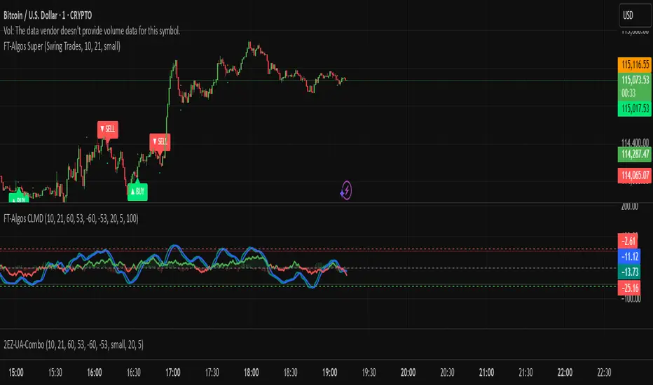
FT-Algos SuperFT-Algos: Unified Alpha Suite
FT-Algos is an all-in-one Pine Script indicator designed to support traders across scalping and swing trading styles with unique multi-strategy logic and clear signals.
Key Features:
Three Trading Modes:
Quick Scalps — Fast momentum-based entries optimized for ultra-short timeframes.
Precision Scalps — Combines MACD flips, Kalman smoothing, Gaussian filters, ZLEMA, and Heikin Ashi SuperTrend to generate high-confidence scalping signals.
Swing Trades — Uses trend stacking with Kalman, ZLEMA, and MACD crossovers confirmed by higher timeframe SuperTrend direction.
Non-Repainting Signals: All entries rely on confirmed candle closes to avoid repainting and false signals.
Visual Entry Markers: Compact BUY and SELL triangle labels placed directly above/below candles for clear signal visualization.
Dynamic Take Profit and Stop Loss Levels: Calculated using Average True Range (ATR) to adjust for current market volatility.
User Configurable Settings: Easily toggle signal visibility, TP/SL display, and short entry signals.
Alert Conditions: Built-in alerts for buy and sell signals enable integration with TradingView’s alert system.
How FT-Algos works:
FT-Algos uniquely blends several filtering methods including Kalman and Gaussian smoothing, momentum evaluation, and multi-timeframe trend validation to minimize noise and improve entry precision. Each mode serves different trading styles—from rapid scalping to higher timeframe swing trading—allowing traders to adapt to their preferred strategy seamlessly.
Disclaimer:
This script is provided as-is for educational and informational purposes only. It does not constitute financial advice. Please test thoroughly and trade responsibly.
חפש סקריפטים עבור "algo"
FT-Algos CLMDFT‑Algos CLMD — Hybrid Momentum & Money Flow Detector
FT‑Algos CLMD is a precision‑built trading tool that blends advanced momentum tracking with dynamic money flow analysis. It provides traders with a clear, dual‑layered view of market strength and potential turning points.
Key Features
Momentum oscillator with overbought/oversold zone markers.
Integrated money flow overlay, scaled for direct visual comparison.
Optional histogram view of momentum differentials.
Adjustable smoothing and scaling controls for full customization.
Automatic positive/negative zone shading for quick sentiment reading.
How It Works
This tool analyzes both momentum shifts and capital flow pressure to highlight moments of potential market imbalance. When both layers align, the probability of a strong move can increase — making it a powerful addition to any trading system.
Notes
Designed for chart analysis; does not execute trades automatically.
Past performance is not indicative of future results.
Always combine with disciplined risk management and other forms of analysis.

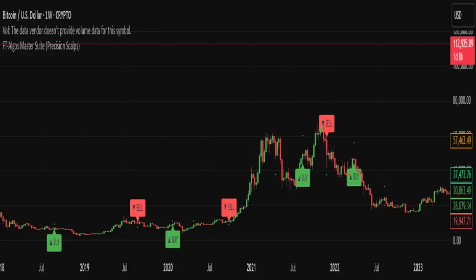
FT-Algos Master SuiteFT-Algos: Unified Alpha Suite
FT-Algos is an all-in-one Pine Script indicator designed to support traders across scalping and swing trading styles with unique multi-strategy logic and clear signals.
Key Features:
Three Trading Modes:
Quick Scalps — Fast momentum-based entries optimized for ultra-short timeframes.
Precision Scalps — Combines MACD flips, Kalman smoothing, Gaussian filters, ZLEMA, and Heikin Ashi SuperTrend to generate high-confidence scalping signals.
Swing Trades — Uses trend stacking with Kalman, ZLEMA, and MACD crossovers confirmed by higher timeframe SuperTrend direction.
Non-Repainting Signals: All entries rely on confirmed candle closes to avoid repainting and false signals.
Visual Entry Markers: Compact BUY and SELL triangle labels placed directly above/below candles for clear signal visualization.
Dynamic Take Profit and Stop Loss Levels: Calculated using Average True Range (ATR) to adjust for current market volatility.
User Configurable Settings: Easily toggle signal visibility, TP/SL display, and short entry signals.
Alert Conditions: Built-in alerts for buy and sell signals enable integration with TradingView’s alert system.
How FT-Algos works:
FT-Algos uniquely blends several filtering methods including Kalman and Gaussian smoothing, momentum evaluation, and multi-timeframe trend validation to minimize noise and improve entry precision. Each mode serves different trading styles—from rapid scalping to higher timeframe swing trading—allowing traders to adapt to their preferred strategy seamlessly.
Disclaimer:
This script is provided as-is for educational and informational purposes only. It does not constitute financial advice. Please test thoroughly and trade responsibly.
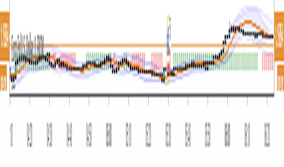
Market Rhythm Trading Algo with Super SignalsThe Market Rhythm trading algo is designed using many different confluence data points that gives you a virtually unlimited combination of settings to manage risk on any given underlying asset. Designed with flexibility in mind, Market Rhythm can be used on futures, stocks, options, and even crypto.
The current settings are what give you the most buy and sell signals. Be sure to change the 'Rate of Change' source to something like hl2 instead of close where it's set to get even more signals.
How to Use:
Regular vs Super - Market Rhythm includes a set of regular signals, which are given on many price bars. Super signals are a combination of regular signals based on a length of bars you set. This is an effective way to clean up the chart and give more reliable buy and sell signals.
The idea behind so many points of confluence is to give you many different ways to filter out the signals you don't want to trade, or just don't like trading. With built in filters using rate of change, rsi, and chop index, you can customize the feel of your signals based on your risk. You can even use the Settings1 and Settings2 and ADX to separate your risk management into 2 different market conditions. For lower ADX settings you can manage risk much tighter for choppier, less trending markets. For higher ADX settings you will be able to set your risk management based on stronger trends.
The Adaptive Average included also changes based on Settings1/2 to give you a better idea of changing market conditions.
The Moving Average Ribbon can be used to temper your decisions for entering or exiting a trade. For instance, if you receive a red (sell signal) during a strong up trend, and the Adaptive Average is green, and the MA Ribbon is all green, then you have a pretty good idea of whether or not its safe to stay in the trade or go ahead and take profit.
Depending on your favorite time frame, Market Rhythm can be used for intraday scalping, as well as, daily swing trading. Not sure if your favorite discord pump stock is ready to go up? Check it against Market Rhythm and you'll have a much better idea of whether it's still going up or if you've missed the move. Trade safer and happier with Market Rhythm.
The small green triangles are 'regular buy signals' and the larger green triangles are 'super buy signals'.
The small red triangles are 'regular sell signals' and the larger red triangles are 'super sell signals'.
Use this indicator against your levels or main strategy for maximum effectiveness.
Limitations:
This script does not mark reversals. It will only identify safe trade zones during periods of strong momentum.
Disclaimer:
The information contained in my scripts/indicators/ideas does not constitute financial advice or a solicitation to buy or sell any securities of any type. I will not accept liability for any loss or damage, including without limitation any loss of profit, which may arise directly or indirectly from the use of or reliance on such information.
All investments involve risk, and the past performance of a security, industry, sector, market, financial product, trading strategy, or individual’s trading does not guarantee future results or returns. Investors are fully responsible for any investment decisions they make. Such decisions should be based solely on an evaluation of their financial circumstances, investment objectives, risk tolerance, and liquidity needs.
My scripts/indicators/strategies/ideas are only for educational purposes!

QaSH DCA AlgorithmQaSH DCA Algorithm implements a DCA strategy that takes advantage of price volatility by buying dips to average down, and adjusting price targets as the break-even price gets lower.
How does the DCA strategy work?
When the specified entry condition has occurred, the indicator will set up several limit orders below the current price. If price goes up a specified amount, then the layers will be overwritten at the higher prices. If price goes down and fills the first layer (limit order), then the Take Profit price is plotted and will be sent in an alert. If more layers are filled, then the TP price will move down accordingly as it’s based on the average entry price (alerts on each TP update). This action of lowering the average entry and TP price mitigates your risk, and increases the likelihood of a Take Profit event happening. More entry conditions will be added as time goes on, although complex entry conditions are not necessary for the strategy to work. All the meat of the DCA strategy is in the layer placement, order volume , and TP %.
How does this differ from other DCA bots?
1) The layer placements, order volume , and “take profit %” for each layer or “safety order” is much more customizable than what you get from other services. For example, I can choose to have my TP% change, depending on how big the price dip was. Maybe on safety order 1 I want 10% TP, but on safety order 7 might want a 2% TP.
2) Settings optimization. You can take advantage of the replay feature and see how trades would have played out, and how much PnL you would have made (strategy version is coming soon)
3) You can use this indicator on more than just crypto. You can easily set up alerts for manual trades on stocks, or you can integrate it with your stock broker API of choice and automate your trades.
4) When combining this with an automation service, you will get unmatched execution speed by running it on your dedicated machine.
5) I can offer a lifetime subscription to the indicator upon request.
What kind of market is it best used on?
QaSH DCA Algorithm is best used on cryptocurrencies and stocks, and it is best used on assets that are volatile. That means large swings up and down. Also I recommend running this on many uncorrelated assets at the same time.
What settings should I use?
The default settings are decent for most markets, and provide a good balance between profit potential and downside protection, although you can use a wide variety of settings. In a strong bull market its best to either bring up your layers to catch smaller dips, or you can go big on the first few layers (maybe 4 layers, 25% on each layer for example). In a sideways or brearish market you'll want more downside protection, so you'll want the larger orders to be at lower prices.
What should I do if price goes below my last layer?
The best solution is to keep a cash reserve on the side at all times. If price looks like it has reached a low point below your lowest layer, then manually buy more to average down further. This action will help it along and get you in the green sooner.
Disclaimer: In order to get a large position in an asset, you need to have most of your layers fill. That means you have to be comfortable with buying more as the price goes down, patiently waiting for the bounce that occurs afterward. This is the working principle of Dollar Cost Averaging, and it's a proven method for most markets.

Dual Thrust Trading Algorithm (ps4)This is an PS4 update to the popular Dual Thrust trading algorithm posted by me some time ago (). It has been commonly used in futures, Forex and equity markets. The idea of Dual Thrust is similar to a typical breakout system, however dual thrust uses the historical price to construct update the look back period - theoretically making it more stable in any given period.
See: www.quantconnect.com

Algo BOT 3.0Algo BOT 3.0 is a sophisticated, rule-based intraday trading strategy designed for index option traders who seek high-probability entries based on market structure, institutional zones, and controlled risk management. This strategy intelligently identifies BUY and SELL trade opportunities using price action, Fibonacci retracements, and pivot confluences, layered with dynamic trade management through trailing stop loss (TSL) and predefined profit/loss thresholds.
🔍 Strategic Foundation
Algo BOT 3.0 combines multiple proven intraday trading concepts into a single unified system:
Candle Behavior Analysis:
Detects strong green (bullish) and red (bearish) candles based on configurable range filters, wick/body ratios, and volume-backed movement.
Ensures only impactful candles are considered for signal generation, filtering out noise.
Dynamic Candle Range Filtering:
Filters out low-momentum candles by comparing their range against a dynamically calculated threshold (based on recent 30-minute close).
Prevents premature or weak entries by focusing on high-volatility structures.
Fibonacci Entry Zones:
Automatically calculates 0.382 and 0.618 Fibonacci levels between the most recent key candles (highest green & lowest red).
These fib levels are used to define entry zones for BUY (above red fib 0.382) and SELL (below green fib 0.382).
Optional fib zones can be visually shown on the chart with real-time drawing.
📈 Signal Generation Logic
The core BUY/SELL signals are triggered based on a combination of:
Green/Red Candle Identification:
A green candle qualifies if:
Open is near the bottom 38.2% of its range.
Close is above the top 61.8% of the range.
High is above a pivot or institutional level.
A red candle qualifies if:
Open is near the top 38.2% of its range.
Close is below the bottom 61.8% of the range.
Low is below a pivot or institutional level.
Support/Resistance Touch Confirmation:
Signals are only considered valid if the qualifying candle touches:
CPR Top/Bottom
Daily Pivot Points (PP, R1–R4, S1–S4)
VWAP or MVWAP
CE Entry (BOT BUY):
Occurs when the price crosses above red fib 0.382 after red candle touch at support.
PE Entry (BOT SELL):
Occurs when the price crosses below green fib 0.382 after green candle touch at resistance.
Signal Controls:
Only one active signal per type (BUY/SELL) at a time.
Real-time tracking of active trade with condition-based resets.
🎯 Exit Management
Built-in risk and profit control with dynamic logic:
Trailing Stop Loss (TSL):
TSL is dynamically adjusted based on peak price after entry.
Trail distance is customizable via input (% below peak).
Visual alerts notify when TSL is hit.
Profit Target:
Trade exits automatically when desired % profit is achieved from entry.
Loss Limit:
Trade exits immediately if unrealized loss exceeds a set % threshold.
Helps prevent large drawdowns during volatile market moves.
🧠 Technical Indicator Integration
To enhance trade accuracy, the strategy includes several optional filters:
RSI: Momentum confirmation or divergence filtering.
SMA/EMA: Trend direction confirmation.
MVWAP: Modified VWAP for smoother institutional bias tracking.
🖼️ Visuals & Alerts
BOT BUY and BOT SELL Signal Labels appear directly on the chart with trade type and candle reference.
TSL, Target, and SL Exits shown as label markers with optional background highlight.
Live Alerts:
BOT BUY (CE Entry)
BOT SELL (PE Entry)
Trailing Stop Loss Triggered
Profit Target Hit
Stop Loss Triggered
⚙️ Customizable Settings
Users can fine-tune the strategy using the following input options:
MVWAP Length
RSI / SMA / EMA Lengths
Candle Range Sensitivity
TSL Distance (%)
Profit Target (%)
Loss Limit (%)
Enable/Disable Background Highlights & Labels
Display Fib Zones
⏱️ Best Use Case & Timeframes

Position and Risk Calculator (for Indices) [dR-Algo]Position and Risk Calculator : Your Ultimate Risk Management Tool for Indices
The difference between a novice and a seasoned trader often comes down to one essential element: risk management. While trading indices, the challenges are even more intense due to market volatility and leverage. The Position and Risk Calculator steps in here to bridge the gap, providing you with an efficient tool designed exclusively for indices trading.
Key Features:
User-Friendly Interface: Designed to integrate effortlessly with your TradingView chart, this tool's interface is intuitive and clutter-free.
Dynamic Price Level Adjustment: Move your Entry, Stop Loss, and Take Profit levels directly on the chart for an interactive experience.
Account Balance Input: Customize the tool to understand your unique financial situation by inputting your current account balance.
Trade Risk Customization: Define how much you're willing to risk per trade, and the tool will do the rest.
Automated Calculations: The indicator calculates the maximum monetary risk and translates it into the maximum lot size you can afford. It delivers a full-integer lot size to make your trading decisions easier.
Comprehensive Risk Evaluation: Beyond lot sizes, it provides you with the Cost-to-Reward Ratio (CRV) of your trade, the actual monetary risk according to the calculated lot size, and the potential profit.
How To Use:
Once you add the Position and Risk Calculator to your TradingView chart, a new interactive panel appears. Here’s how it works:
Set Price Levels: Using draggable lines on the chart, set your Entry Price, Stop Loss, and Take Profit levels.
Account Details: Go to settings and enter your Account Balance and your desired risk percentage per trade.
Automatic Calculations: As soon as the above details are set, the indicator goes to work. It first calculates your maximum risk in monetary terms and then translates that into the maximum lot size you can take for the trade.
Review and Trade: The indicator shows you all the vital statistics - CRV of the trade, the money at risk according to the calculated lot size, and the possible profit.
Why Choose This Tool?
Informed Decisions: Your trading decisions will be based on concrete numbers, removing guesswork.
Time-saving: No need for manual calculations or using separate tools; everything is in one place.
Focus on Trading: By automating the risk management aspect, this tool allows you to focus more on your trading strategy and market analysis.
Tailor-Made for Indices: Unlike many other tools that try to serve all markets, the Position and Risk Calculator is designed specifically for indices trading.
Remember, effective risk management is what separates successful traders from those who burn out. The Position and Risk Calculator not only helps you define your risk but also helps you understand it, empowering you to trade with confidence.
So why not give yourself the best chance of success? Add the Position and Risk Calculator to your TradingView setup and experience the difference it can make.

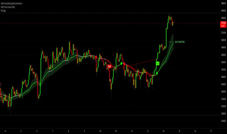
RSI Algo (Pinescript v5 + Alerts)Found this the other day and thought it might be useful to have an updated version with alerts:
Credit to the original author.
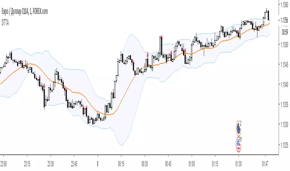
Cluster Algo (Skoda Version)This Indicator operates similarly to the Cluster Algo marketed elsewhere. The key difference is the integration of Bollinger Bands, giving us clear indications.
Buy - When the signal line goes above the Bollinger basis line and is GREEN
Sell - When the signal line goes below the Bollinger basis line and is RED
Consider closing the trade when the signal line changes colour.
When the signal line goes outside the Bollinger band, this a strong indication price will rally.
If you require any further information or script modifications, please message me.
PLEASE CHECK OUT MY OTHER SCRIPTS


Dual Thrust Trading AlgorithmThe Dual Thrust trading algorithm is a famous strategy developed by Michael Chalek. It has been commonly used in futures, forex and equity markets. The idea of Dual Thrust is similar to a typical breakout system, however dual thrust uses the historical price to construct update the look back period - theoretically making it more stable in any given period.
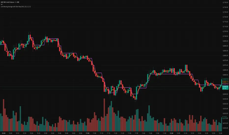
Jurik Moving Average with Stair-StepJurik Moving Average with Stair-Step Filter — Precision Smoothing with Event-Driven Signal Filtering
📌 Version:
Built in Pine Script v6, leveraging the full JMA core with an added stair-step threshold filter for discrete, event-based signal generation.
📌 Overview:
This enhanced Jurik Moving Average (JMA) combines the low-lag smoothing algorithm with a custom stair-step logic layer that transforms continuous JMA output into state-based, noise-filtered movement.
While the traditional JMA provides ultra-smooth, adaptive trend detection, it still updates continuously with each price tick. The Stair-Step version introduces a quantized output — the JMA value remains unchanged until price moves by a user-defined amount (in ticks or absolute price units). The result is a “digital” trend line that updates only when meaningful change occurs, filtering out minor fluctuations and giving traders clearer, more actionable transitions.
📌 How It Works:
✅ Adaptive JMA Core: Dynamically adjusts smoothing to volatility for ultra-low lag.
✅ Stair-Step Logic: Holds the JMA value steady until the underlying line moves by a chosen threshold.
✅ Event-Driven Updates: Each “step” represents a statistically significant change in market direction.
✅ Tick / Price-Based Sensitivity: Tune the filter to the instrument’s volatility, spread, or cost structure.
This dual-layer system blends JMA’s continuous adaptability with discrete regime detection — turning a smooth line into a decision-ready trend model.
📌 How to Use:
🔹 Bias Detection: Each new step indicates a potential regime shift or breakout confirmation.
🔹 Noise Reduction: Ideal in choppy or range-bound markets where traditional MAs over-react.
🔹 Automated Systems: Use stair transitions as clean event triggers for entries, exits, or bias flips.
🔹 Scalping & Swing Trading: Thresholds can be sized by tick, ATR, or volatility to match timeframe and cost tolerance.
📌 Why This Version Is Unique:
This is not just another moving average — it’s a stateful JMA, adding event-driven decision logic to one of the market’s most precise filters.
🔹 Discretized Trend Mapping: Flat plateaus define stability; steps define momentum bursts.
🔹 Reduced Whipsaws: Only reacts when moves exceed statistical or cost thresholds.
🔹 Execution-Grade Precision: Perfect for algorithmic strategies needing fewer false flips.
📌 Example Use:
Combine with VWAP, ATR, or momentum oscillators to confirm bias shifts. In automated strategies, use stair flips as “go / stop” states to control position changes or trade size adjustments.
📌 Summary:
The Jurik Moving Average with Stair-Step Filter preserves JMA’s hallmark smoothness while delivering a structured, event-driven representation of market movement.
It’s precision smoothing — now with adaptive noise gating — designed for traders who demand clarity, stability, and algorithm-ready signal behavior.
📌 Disclaimer:
This indicator is not affiliated with or derived from any proprietary Jurik Research algorithms. It’s an independent implementation that applies similar adaptive-smoothing principles, extended with a stair-step filtering mechanism for discrete trend transitions.
Periodis ProIntroduction
The Algorion Periodis Pro represents a paradigm shift in professional trend analysis. Unlike traditional indicators that force the market to fit into rigid, pre-defined settings (like a 14-period MA), this system allows the market to dictate its own parameters.
By combining a Proprietary Anchored Framework with specific temporal resets, Algorion Periodis Pro captures the "natural rhythm" of price action, offering a view of the market that is mathematically synchronized with the current trading session, day, or week.
Core Methodology: The "Zero-Parameter" Philosophy
The true power of Algorion Periodis Pro lies in its unique approach to signal generation. It does not rely on arbitrary user inputs. Instead, it features two distinct, self-adaptive lines that construct themselves in real-time:
1. The Self-Constructing Inertia Line (Adaptive EMA): This line is not calculated using a fixed lookback period. Instead, it builds itself from the ground up starting at each reset point. It accepts the market’s raw price action as its sole instruction set, naturally deriving its own smoothing coefficients based on the speed and flow of the current trend. It represents the market’s "Inertia."
2. The Proprietary Efficiency Filter: The second line utilizes a highly advanced, parameter-free algorithm. It "listens" to the market's noise and volatility levels to determine its own sensitivity. When price is clean, it tightens; when price is chaotic, it relaxes.
The Result: Two lines that are not imposed on the market, but are born from the market. Their interaction reveals the true fair value without the lag caused by human bias.
Features & Functionality
The "Heartbeat" of Volatility (Heatmap Bands): Standard deviation bands often lag. Algorion Periodis Pro, however, calculates the Accumulated Volatility from the anchor point.
These bands represent the "breathing room" the market requires for the current period.
Info Box Dashboard: The panel in the corner displays the Base Volatility State. This value (measured in Ticks/Pips/Points) is the precise distance between the Main Line and the first Deviation Band. This is the current "Volatility Unit" of the asset.
Dual-Set Chronology:
Set 1 (Tactical): Captures the immediate, intraday pulse (Default: 600 Minutes).
Set 2 (Strategic): Captures the broader structural intent (Default: Weekly).
Smart Confluence Coloring: Bars are painted Green or Red only when a "Council of Factors"—including the slopes of both adaptive lines and internal trend metrics—agree on the direction. This filters out weak, non-committal price action.
Strategic Usage: Volatility-Synchronized Trading
Because the Deviation Bands are derived from the market's natural volatility accumulation, they serve as the perfect coordinate system for Risk Management:
Risk (Stop Loss): Use the Base Volatility Unit (the distance of one band) as your natural stop-loss distance. This places your stop outside the current "noise floor" of the market.
Reward (Targets): Target the outer bands.
Band 1-2: High-probability scalping targets during standard moves.
Band 3+: Targets for expansion moves.
Level-to-Level Trading: In a trending market, price often climbs the "ladder" of these bands. A breakout above Band 1 often targets Band 2. When price extends to the outer limits (Band 6 or 7), it often signals a statistical exhaustion, offering a mean-reversion opportunity back to the Main Line.
Configuration
Main Line Switches: Toggle the Main and Secondary lines On/Off for both sets to suit your visual preference.
Reset Frequency: Define the life-cycle of the calculation (Minutes, Daily, Weekly).
Confluence Threshold: Adjust the strictness of the Bar Coloring (voting factors).
Signal Markers: Toggle discrete Buy/Sell shapes based on the structural trend.
Disclaimer
This tool is for informational purposes only. The proprietary algorithms contained herein calculate derived values from past price action and cannot predict future market movements with certainty. Past performance is not indicative of future results. Always manage risk.

AK MACD BB INDICATOR V 1.00Here's my version of the MACD _BB . This is a great indicator to capture short term trends.
yellow candles = long
aqua candles = short
This indicator can be much better. I will work on it and publish an improved version (hopefully) soon. In the mean time , go ahead and play around with the code, and please share your findings :)
Cheers
Algo

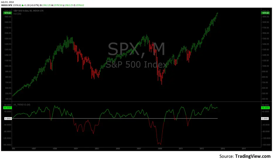
AK TREND ID v1.00Hello,
"Are we at the top yet ? "........ " Is it a good time to invest ? " ......." Should I buy or sell ? " These are the many questions I hear and get on the daily basis. 1000's of investors do not know when to go in and out of the market. Most of them rely on the opinion of "experts" on television to make their investment decisions. Bad idea.Taking a systematic approach when investing, could save you a lot of time and headache. If there was only a way to know when to get in and out of the market !! hmmmm. The good news is that there many ways to do that. The bad news is , are you disciplined enough to follow it ?
I coded the AK_TREND ID specifically to identified trends in the SPX or SPY only . How does it work ? very simply , I simply plot the spread between the 3 month and 8 month moving average on the chart.
If the spread > 0 @ month end = BUY
if the spread < 0 @ month end = SELL
The AK TREND ID is a LAGGING Indicator , so it will not get you in at the very bottom or get you out at the very top. I did a backtest on the SPX from 1984 to 7/2/2014 (yesterday), The rule was to buy only when the AK TREND ID was green. let's look at the result:
14 trades : 11 W 3 L , 78.75 % winning %
Biggest winner (%) = 108 %
Biggest loser (%) = -10.7 %
Average Return = 27 %
Total Return since 1984 = 351.3 %
You can see the result in detail here : docs.google.com
Although the backtesting results are good, the AK TREND ID is not to be used as a trading system. It is simply design to let you know when to invest and when to get out. I'm working a more accurate version of this Indicator , that will use both technical and fundamental data. In the mean time , I hope this will give some of you piece of mind, and eliminate emotions from your trading decision. Feel free to modify the code as you wish, but please share your finding with the rest of Trading View community.
All the best
Algo
Risk Recommender — (Heatmap)📊 Risk Recommender — Per-Trade & Annualized (Heatmap Columns)
Estimate the optimal risk percentage for any market regime.
This tool dynamically recommends how much of your account equity to risk — either per trade or at a portfolio (annualized) level — using volatility as the guide.
⚙️ How it works
Two distinct modes give you flexibility:
1️⃣ Per-Trade (ATR-based)
• Calculates the current Average True Range (ATR) compared to its long-term baseline.
• When volatility is high (ATR ↑), risk per trade decreases to maintain constant dollar risk.
• When volatility is low (ATR ↓), risk per trade increases within your defined floor and ceiling.
• The display is normalized by stop distance (× ATR) and smoothed to avoid noise.
2️⃣ Annualized (Volatility Targeting)
• Computes realized volatility (standard deviation of log returns) and an EWMA forecast of future volatility.
• Blends current and forecast volatilities to estimate “effective” volatility.
• Scales your base risk so that portfolio volatility converges toward your chosen annual target (e.g., 20%).
• Useful for portfolio-level or systematic strategies that maintain constant volatility exposure.
🎨 Heatmap Visualization
The vertical column graph acts like a thermometer:
• 🟥 Red → “Reduce risk” (volatility high).
• 🟩 Green → “Increase risk” (volatility low).
• Smoothed and bounded between your Floor and Ceiling risk levels.
• Optional dotted guides mark those bounds.
• Label shows the current mode, recommended risk %, and key metrics (ATR ratio or effective volatility).
🔧 Key Inputs
• Base max risk per trade (%) — your normal per-trade risk budget.
• ATR length / Baseline ATR length — control sensitivity to short- vs. long-term volatility.
• Target annualized volatility (%) — portfolio volatility target for quant mode.
• λ (lambda) — smoothing factor for the EWMA volatility forecast (0.90–0.99 typical).
• Floor & Ceiling — clamps the output to avoid extreme sizing.
• Smoothing & Hysteresis — prevent rapid changes in risk recommendations.
🧮 Interpreting the Output
• “Recommended Risk (%)” = suggested portion of equity to risk on the next trade (or current exposure).
• In Per-Trade mode: reflects current ATR ÷ baseline ATR .
• In Annualized mode: reflects target volatility ÷ effective volatility .
• Use the color and height of the column as a quick visual cue for aggressiveness.
💡 Typical Use Cases
• Position-sizing overlay for discretionary traders.
• Volatility-targeting component for algorithmic or multi-asset systems.
• Educational tool to understand how volatility governs prudent risk management.
📘 Notes
• This indicator provides risk suggestions only ; it does not place trades.
• Works on any symbol or timeframe.
• Combine with your own strategy or alerts for full automation.
• All calculations use built-in Pine functions; no proprietary logic.
Tags:
#RiskManagement #ATR #Volatility #Quant #PositionSizing #SystematicTrading #AlgorithmicTrading #Portfolio #TradingStrategy #Heatmap #EWMA #Risk

Jurik Moving AverageJurik Moving Average (JMA) – Precision Smoothing with Adaptive Filtering
📌 Version: This script is written in Pine Script v6, utilizing advanced array handling and dynamic filtering for improved performance.
📌 Overview:
The Jurik Moving Average (JMA) was originally developed by Mark Jurik and is widely recognized for its ability to provide smooth trend-following signals with minimal lag. Unlike traditional moving averages, which suffer from a tradeoff between responsiveness and smoothness, JMA employs an adaptive smoothing algorithm that dynamically adjusts based on market conditions, reducing false signals while maintaining trend accuracy.
This version of JMA has been implemented in Pine Script v6 with enhancements that make it even more efficient for TradingView users. By utilizing advanced array-based calculations, logarithmic scaling, and cycle-based filtering, this implementation delivers an optimized, customizable, and high-performance smoothing indicator.
📌 How It Works:
✅ Adaptive Filtering: Dynamically adjusts smoothing based on price volatility.
✅ Cycle-Based Adjustments: Uses historical price action to fine-tune lag vs. responsiveness.
✅ Advanced Phase Control: Traders can shift the moving average forward or backward to optimize signal alignment.
Unlike existing open-source JMA implementations, this version features:
🔹 Enhanced Array-Based Calculations for better memory management & performance.
🔹 Logarithmic and Square Root Scaling to dynamically adjust phase & smoothing.
🔹 Improved Noise Reduction Techniques to minimize false breakouts.
📌 How to Use:
🔹 Trend Confirmation: Use JMA to validate trend direction and avoid whipsaws.
🔹 Trade Entries & Exits: Combine with price action or momentum indicators for refined entry/exit points.
🔹 Scalping & Swing Trading: Ideal for short-term and long-term strategies due to its adaptability.
📌 Why This Version is Unique:
This JMA expands on standard implementations by incorporating multi-level cycle smoothing, phase correction, and adaptive noise filtering. The result? A more precise, stable, and robust trend indicator that performs better than existing open-source versions.

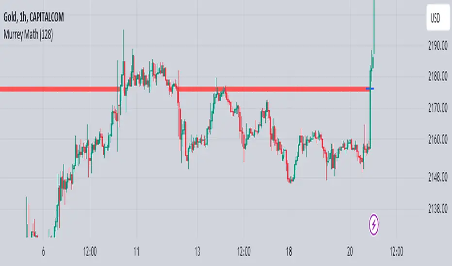
Murrey Math
The Murrey Math indicator is a set of horizontal price levels, calculated from an algorithm developed by stock trader T.J. Murray.
The main concept behind Murrey Math is that prices tend to react and rotate at specific price levels. These levels are calculated by dividing the price range into fixed segments called "ranges", usually using a number of 8, 16, 32, 64, 128 or 256.
Murrey Math levels are calculated as follows:
1. A particular price range is taken, for example, 128.
2. Divide the current price by the range (128 in this example).
3. The result is rounded to the nearest whole number.
4. Multiply that whole number by the original range (128).
This results in the Murrey Math level closest to the current price. More Murrey levels are calculated and drawn by adding and subtracting multiples of the range to the initially calculated level.
Traders use Murrey Math levels as areas of possible support and resistance as it is believed that prices tend to react and pivot at these levels. They are also used to identify price patterns and possible entry and exit points in trading.
The Murrey Math indicator itself simply calculates and draws these horizontal levels on the price chart, allowing traders to easily visualize them and use them in their technical analysis.
HOW TO USE THIS INDICATOR?
To use the Murrey Math indicator effectively, here are some tips:
1. Choose the appropriate Murrey Math range : The Murrey Math range input (128 by default in the provided code) determines the spacing between the levels. Common ranges used are 8, 16, 32, 64, 128, and 256. A smaller range will give you more levels, while a larger range will give you fewer levels. Choose a range that suits the volatility and trading timeframe you're working with.
2. Identify potential support and resistance levels: The horizontal lines drawn by the indicator represent potential support and resistance levels based on the Murrey Math calculation. Prices often react or reverse at these levels, so they can be used to spot areas of interest for entries and exits.
3. Look for price reactions at the levels: Watch for price action like rejections, bounces, or breakouts at the Murrey Math levels. These reactions can signal potential trend continuation or reversal setups.
4. Trail stop-loss orders: You can place stop-loss orders just below/above the nearest Murrey Math level to manage risk if the price moves against your trade.
5. Set targets at future levels: Project potential profit targets by looking at upcoming Murrey Math levels in the direction of the trend.
7. Adjust range as needed: If prices are consistently breaking through levels without reacting, try adjusting the range input to a different value to see if it provides better levels.
In which asset can this indicator perform better?
The Murrey Math indicator can potentially perform well on any liquid financial asset that exhibits some degree of mean-reversion or trading range behavior. However, it may be more suitable for certain asset classes or trading timeframes than others.
Here are some assets and scenarios where the Murrey Math indicator can potentially perform better:
1. Forex Markets: The foreign exchange market is known for its ranging and mean-reverting nature, especially on higher timeframes like the daily or weekly charts. The Murrey Math levels can help identify potential support and resistance levels within these trading ranges.
2. Futures Markets: Futures contracts, such as those for commodities (e.g., crude oil, gold, etc.) or equity indices, often exhibit trading ranges and mean-reversion trends. The Murrey Math indicator can be useful in identifying potential turning points within these ranges.
3. Stocks with Range-bound Behavior: Some stocks, particularly those of large-cap companies, can trade within well-defined ranges for extended periods. The Murrey Math levels can help identify the boundaries of these ranges and potential reversal points.
4. I ntraday Trading: The Murrey Math indicator may be more effective on lower timeframes (e.g., 1-hour, 30-minute, 15-minute) for intraday trading, as prices tend to respect support and resistance levels more closely within shorter time periods.
5. Trending Markets: While the Murrey Math indicator is primarily designed for range-bound markets, it can also be used in trending markets to identify potential pullback or continuation levels.

Algorithm Predator - ProAlgorithm Predator - Pro: Advanced Multi-Agent Reinforcement Learning Trading System
Algorithm Predator - Pro combines four specialized market microstructure agents with a state-of-the-art reinforcement learning framework . Unlike traditional indicator mashups, this system implements genuine machine learning to automatically discover which detection strategies work best in current market conditions and adapts continuously without manual intervention.
Core Innovation: Rather than forcing traders to interpret conflicting signals, this system uses 15 different multi-armed bandit algorithms and a full reinforcement learning stack (Q-Learning, TD(λ) with eligibility traces, and Policy Gradient with REINFORCE) to learn optimal agent selection policies. The result is a self-improving system that gets smarter with every trade.
Target Users: Swing traders, day traders, and algorithmic traders seeking systematic signal generation with mathematical rigor. Suitable for stocks, forex, crypto, and futures on liquid instruments (>100k daily volume).
Why These Components Are Combined
The Fundamental Problem
No single indicator works consistently across all market regimes. What works in trending markets fails in ranging conditions. Traditional solutions force traders to manually switch indicators (slow, error-prone) or interpret all signals simultaneously (cognitive overload).
This system solves the problem through automated meta-learning: Deploy multiple specialized agents designed for specific market microstructure conditions, then use reinforcement learning to discover which agent (or combination) performs best in real-time.
Why These Specific Four Agents?
The four agents provide orthogonal failure mode coverage —each agent's weakness is another's strength:
Spoofing Detector - Optimal in consolidation/manipulation; fails in trending markets (hedged by Exhaustion Detector)
Exhaustion Detector - Optimal at trend climax; fails in range-bound markets (hedged by Liquidity Void)
Liquidity Void - Optimal pre-breakout compression; fails in established trends (hedged by Mean Reversion)
Mean Reversion - Optimal in low volatility; fails in strong trends (hedged by Spoofing Detector)
This creates complete market state coverage where at least one agent should perform well in any condition. The bandit system identifies which one without human intervention.
Why Reinforcement Learning vs. Simple Voting?
Traditional consensus systems have fatal flaws: equal weighting assumes all agents are equally reliable (false), static thresholds don't adapt, and no learning means past mistakes repeat indefinitely.
Reinforcement learning solves this through the exploration-exploitation tradeoff: Continuously test underused agents (exploration) while primarily relying on proven winners (exploitation). Over time, the system builds a probability distribution over agent quality reflecting actual market performance.
Mathematical Foundation: Multi-armed bandit problem from probability theory, where each agent is an "arm" with unknown reward distribution. The goal is to maximize cumulative reward while efficiently learning each arm's true quality.
The Four Trading Agents: Technical Explanation
Agent 1: 🎭 Spoofing Detector (Institutional Manipulation Detection)
Theoretical Basis: Market microstructure theory on order flow toxicity and information asymmetry. Based on research by Easley, López de Prado, and O'Hara on high-frequency trading manipulation.
What It Detects:
1. Iceberg Orders (Hidden Liquidity Absorption)
Method: Monitors volume spikes (>2.5× 20-period average) with minimal price movement (<0.3× ATR)
Formula: score += (close > open ? -2.5 : 2.5) when volume > vol_avg × 2.5 AND abs(close - open) / ATR < 0.3
Interpretation: Large volume without price movement indicates institutional absorption (buying) or distribution (selling) using hidden orders
Signal Logic: Contrarian—fade false breakouts caused by institutional manipulation
2. Spoofing Patterns (Fake Liquidity via Layering)
Method: Analyzes candlestick wick-to-body ratios during volume spikes
Formula: if upper_wick > body × 2 AND volume_spike: score += 2.0
Mechanism: Spoofing creates large wicks (orders pulled before execution) with volume evidence
Signal Logic: Wick direction indicates trapped participants; trade against the failed move
3. Post-Manipulation Reversals
Method: Tracks volume decay after manipulation events
Formula: if volume > vol_avg × 3 AND volume / volume < 0.3: score += (close > open ? -1.5 : 1.5)
Interpretation: Sharp volume drop after manipulation indicates exhaustion of manipulative orders
Why It Works: Institutional manipulation creates detectable microstructure anomalies. While retail traders see "mysterious reversals," this agent quantifies the order flow patterns causing them.
Parameter: i_spoof (sensitivity 0.5-2.0) - Controls detection threshold
Best Markets: Consolidations before breakouts, London/NY overlap windows, stocks with institutional ownership >70%
Agent 2: ⚡ Exhaustion Detector (Momentum Failure Analysis)
Theoretical Basis: Technical analysis divergence theory combined with VPIN reversals from market microstructure literature.
What It Detects:
1. Price-RSI Divergence (Momentum Deceleration)
Method: Compares 5-bar price ROC against RSI change
Formula: if price_roc > 5% AND rsi_current < rsi : score += 1.8
Mathematics: Second derivative detecting inflection points
Signal Logic: When price makes higher highs but momentum makes lower highs, expect mean reversion
2. Volume Exhaustion (Buying/Selling Climax)
Method: Identifies strong price moves (>5% ROC) with declining volume (<-20% volume ROC)
Formula: if price_roc > 5 AND vol_roc < -20: score += 2.5
Interpretation: Price extension without volume support indicates retail chasing while institutions exit
3. Momentum Deceleration (Acceleration Analysis)
Method: Compares recent 3-bar momentum to prior 3-bar momentum
Formula: deceleration = abs(mom1) < abs(mom2) × 0.5 where momentum significant (> ATR)
Signal Logic: When rate of price change decelerates significantly, anticipate directional shift
Why It Works: Momentum is lagging, but momentum divergence is leading. By comparing momentum's rate of change to price, this agent detects "weakening conviction" before reversals become obvious.
Parameter: i_momentum (sensitivity 0.5-2.0)
Best Markets: Strong trends reaching climax, parabolic moves, instruments with high retail participation
Agent 3: 💧 Liquidity Void Detector (Breakout Anticipation)
Theoretical Basis: Market liquidity theory and order book dynamics. Based on research into "liquidity holes" and volatility compression preceding expansion.
What It Detects:
1. Bollinger Band Squeeze (Volatility Compression)
Method: Monitors Bollinger Band width relative to 50-period average
Formula: bb_width = (upper_band - lower_band) / middle_band; triggers when < 0.6× average
Mathematical Foundation: Regression to the mean—low volatility precedes high volatility
Signal Logic: When volatility compresses AND cumulative delta shows directional bias, anticipate breakout
2. Volume Profile Gaps (Thin Liquidity Zones)
Method: Identifies sharp volume transitions indicating few limit orders
Formula: if volume < vol_avg × 0.5 AND volume < vol_avg × 0.5 AND volume > vol_avg × 1.5
Interpretation: Sudden volume drop after spike indicates price moved through order book to low-opposition area
Signal Logic: Price accelerates through low-liquidity zones
3. Stop Hunts (Liquidity Grabs Before Reversals)
Method: Detects new 20-bar highs/lows with immediate reversal and rejection wick
Formula: if new_high AND close < high - (high - low) × 0.6: score += 3.0
Mechanism: Market makers push price to trigger stop-loss clusters, then reverse
Signal Logic: Enter reversal after stop-hunt completes
Why It Works: Order book theory shows price moves fastest through zones with minimal liquidity. By identifying these zones before major moves, this agent provides early entry for high-reward breakouts.
Parameter: i_liquidity (sensitivity 0.5-2.0)
Best Markets: Range-bound pre-breakout setups, volatility compression zones, instruments prone to gap moves
Agent 4: 📊 Mean Reversion (Statistical Arbitrage Engine)
Theoretical Basis: Statistical arbitrage theory, Ornstein-Uhlenbeck mean-reverting processes, and pairs trading methodology applied to single instruments.
What It Detects:
1. Z-Score Extremes (Standard Deviation Analysis)
Method: Calculates price distance from 20-period and 50-period SMAs in standard deviation units
Formula: zscore_20 = (close - SMA20) / StdDev(50)
Statistical Interpretation: Z-score >2.0 means price is 2 standard deviations above mean (97.5th percentile)
Trigger Logic: if abs(zscore_20) > 2.0: score += zscore_20 > 0 ? -1.5 : 1.5 (fade extremes)
2. Ornstein-Uhlenbeck Process (Mean-Reverting Stochastic Model)
Method: Models price as mean-reverting stochastic process: dx = θ(μ - x)dt + σdW
Implementation: Calculates spread = close - SMA20, then z-score of spread vs. spread distribution
Formula: ou_signal = (spread - spread_mean) / spread_std
Interpretation: Measures "tension" pulling price back to equilibrium
3. Correlation Breakdown (Regime Change Detection)
Method: Compares 50-period price-volume correlation to 10-period correlation
Formula: corr_breakdown = abs(typical_corr - recent_corr) > 0.5
Enhancement: if corr_breakdown AND abs(zscore_20) > 1.0: score += zscore_20 > 0 ? -1.2 : 1.2
Why It Works: Mean reversion is the oldest quantitative strategy (1970s pairs trading at Morgan Stanley). While simple, it remains effective because markets exhibit periodic equilibrium-seeking behavior. This agent applies rigorous statistical testing to identify when mean reversion probability is highest.
Parameter: i_statarb (sensitivity 0.5-2.0)
Best Markets: Range-bound instruments, low-volatility periods (VIX <15), algo-dominated markets (forex majors, index futures)
Multi-Armed Bandit System: 15 Algorithms Explained
What Is a Multi-Armed Bandit Problem?
Origin: Named after slot machines ("one-armed bandits"). Imagine facing multiple slot machines, each with unknown payout rates. How do you maximize winnings?
Formal Definition: K arms (agents), each with unknown reward distribution with mean μᵢ. Goal: Maximize cumulative reward over T trials. Challenge: Balance exploration (trying uncertain arms to learn quality) vs. exploitation (using known-best arm for immediate reward).
Trading Application: Each agent is an "arm." After each trade, receive reward (P&L). Must decide which agent to trust for next signal.
Algorithm Categories
Bayesian Approaches (probabilistic, optimal for stationary environments):
Thompson Sampling
Bootstrapped Thompson Sampling
Discounted Thompson Sampling
Frequentist Approaches (confidence intervals, deterministic):
UCB1
UCB1-Tuned
KL-UCB
SW-UCB (Sliding Window)
D-UCB (Discounted)
Adversarial Approaches (robust to non-stationary environments):
EXP3-IX
Hedge
FPL-Gumbel
Reinforcement Learning Approaches (leverage learned state-action values):
Q-Values (from Q-Learning)
Policy Network (from Policy Gradient)
Simple Baseline:
Epsilon-Greedy
Softmax
Key Algorithm Details
Thompson Sampling (DEFAULT - RECOMMENDED)
Theoretical Foundation: Bayesian decision theory with conjugate priors. Published by Thompson (1933), rediscovered for bandits by Chapelle & Li (2011).
How It Works:
Model each agent's reward distribution as Beta(α, β) where α = wins, β = losses
Each step, sample from each agent's beta distribution: θᵢ ~ Beta(αᵢ, βᵢ)
Select agent with highest sample: argmaxᵢ θᵢ
Update winner's distribution after observing outcome
Mathematical Properties:
Optimality: Achieves logarithmic regret O(K log T) (proven optimal)
Bayesian: Maintains probability distribution over true arm means
Automatic Balance: High uncertainty → more exploration; high certainty → exploitation
⚠️ CRITICAL APPROXIMATION: This is a pseudo-random approximation of true Thompson Sampling. True implementation requires random number generation from beta distributions, which Pine Script doesn't provide. This version uses Box-Muller transform with market data (price/volume decimal digits) as entropy source. While not mathematically pure, it maintains core exploration-exploitation balance and learns agent preferences effectively.
When To Use: Best all-around choice. Handles non-stationary markets reasonably well, balances exploration naturally, highly sample-efficient.
UCB1 (Upper Confidence Bound)
Formula: UCB_i = reward_mean_i + sqrt(2 × ln(total_pulls) / pulls_i)
Interpretation: First term (exploitation) + second term (exploration bonus for less-tested arms)
Mathematical Properties:
Deterministic : Always selects same arm given same state
Regret Bound: O(K log T) — same optimality as Thompson Sampling
Interpretable: Can visualize confidence intervals
When To Use: Prefer deterministic behavior, want to visualize uncertainty, stable markets
EXP3-IX (Exponential Weights - Adversarial)
Theoretical Foundation: Adversarial bandit algorithm. Assumes environment may be actively hostile (worst-case analysis).
How It Works:
Maintain exponential weights: w_i = exp(η × cumulative_reward_i)
Select agent with probability proportional to weights: p_i = (1-γ)w_i/Σw_j + γ/K
After outcome, update with importance weighting: estimated_reward = observed_reward / p_i
Mathematical Properties:
Adversarial Regret: O(sqrt(TK log K)) even if environment is adversarial
No Assumptions: Doesn't assume stationary or stochastic reward distributions
Robust: Works even when optimal arm changes continuously
When To Use: Extreme non-stationarity, don't trust reward distribution assumptions, want robustness over efficiency
KL-UCB (Kullback-Leibler Upper Confidence Bound)
Theoretical Foundation: Uses KL-divergence instead of Hoeffding bounds. Tighter confidence intervals.
Formula (conceptual): Find largest q such that: n × KL(p||q) ≤ ln(t) + 3×ln(ln(t))
Mathematical Properties:
Tighter Bounds: KL-divergence adapts to reward distribution shape
Asymptotically Optimal: Better constant factors than UCB1
Computationally Intensive: Requires iterative binary search (15 iterations)
When To Use: Maximum sample efficiency needed, willing to pay computational cost, long-term trading (>500 bars)
Q-Values & Policy Network (RL-Based Selection)
Unique Feature: Instead of treating agents as black boxes with scalar rewards, these algorithms leverage the full RL state representation .
Q-Values Selection:
Uses learned Q-values: Q(state, agent_i) from Q-Learning
Selects agent via softmax over Q-values for current market state
Advantage: Selects based on state-conditional quality (which agent works best in THIS market state)
Policy Network Selection:
Uses neural network policy: π(agent | state, θ) from Policy Gradient
Direct policy over agents given market features
Advantage: Can learn non-linear relationships between market features and agent quality
When To Use: After 200+ RL updates (Q-Values) or 500+ updates (Policy Network) when models converged
Machine Learning & Reinforcement Learning Stack
Why Both Bandits AND Reinforcement Learning?
Critical Distinction:
Bandits treat agents as contextless black boxes: "Agent 2 has 60% win rate"
Reinforcement Learning adds state context: "Agent 2 has 60% win rate WHEN trend_score > 2 and RSI < 40"
Power of Combination: Bandits provide fast initial learning with minimal assumptions. RL provides state-dependent policies for superior long-term performance.
Component 1: Q-Learning (Value-Based RL)
Algorithm: Temporal Difference Learning with Bellman equation.
State Space: 54 discrete states formed from:
trend_state = {0: bearish, 1: neutral, 2: bullish} (3 values)
volatility_state = {0: low, 1: normal, 2: high} (3 values)
RSI_state = {0: oversold, 1: neutral, 2: overbought} (3 values)
volume_state = {0: low, 1: high} (2 values)
Total states: 3 × 3 × 3 × 2 = 54 states
Action Space: 5 actions (No trade, Agent 1, Agent 2, Agent 3, Agent 4)
Total state-action pairs: 54 × 5 = 270 Q-values
Bellman Equation:
Q(s,a) ← Q(s,a) + α ×
Parameters:
α (learning rate): 0.01-0.50, default 0.10 - Controls step size for updates
γ (discount factor): 0.80-0.99, default 0.95 - Values future rewards
ε (exploration): 0.01-0.30, default 0.10 - Probability of random action
Update Mechanism:
Position opens with state s, action a (selected agent)
Every bar position is open: Calculate floating P&L → scale to reward
Perform online TD update
When position closes: Perform terminal update with final reward
Gradient Clipping: TD errors clipped to ; Q-values clipped to for stability.
Why It Works: Q-Learning learns "quality" of each agent in each market state through trial and error. Over time, builds complete state-action value function enabling optimal state-dependent agent selection.
Component 2: TD(λ) Learning (Temporal Difference with Eligibility Traces)
Enhancement Over Basic Q-Learning: Credit assignment across multiple time steps.
The Problem TD(λ) Solves:
Position opens at t=0
Market moves favorably at t=3
Position closes at t=8
Question: Which earlier decisions contributed to success?
Basic Q-Learning: Only updates Q(s₈, a₈) ← reward
TD(λ): Updates ALL visited state-action pairs with decayed credit
Eligibility Trace Formula:
e(s,a) ← γ × λ × e(s,a) for all s,a (decay all traces)
e(s_current, a_current) ← 1 (reset current trace)
Q(s,a) ← Q(s,a) + α × TD_error × e(s,a) (update all with trace weight)
Lambda Parameter (λ): 0.5-0.99, default 0.90
λ=0: Pure 1-step TD (only immediate next state)
λ=1: Full Monte Carlo (entire episode)
λ=0.9: Balance (recommended)
Why Superior: Dramatically faster learning for multi-step tasks. Q-Learning requires many episodes to propagate rewards backwards; TD(λ) does it in one.
Component 3: Policy Gradient (REINFORCE with Baseline)
Paradigm Shift: Instead of learning value function Q(s,a), directly learn policy π(a|s).
Policy Network Architecture:
Input: 12 market features
Hidden: None (linear policy)
Output: 5 actions (softmax distribution)
Total parameters: 12 features × 5 actions + 5 biases = 65 parameters
Feature Set (12 Features):
Price Z-score (close - SMA20) / ATR
Volume ratio (volume / vol_avg - 1)
RSI deviation (RSI - 50) / 50
Bollinger width ratio
Trend score / 4 (normalized)
VWAP deviation
5-bar price ROC
5-bar volume ROC
Range/ATR ratio - 1
Price-volume correlation (20-period)
Volatility ratio (ATR / ATR_avg - 1)
EMA50 deviation
REINFORCE Update Rule:
θ ← θ + α × ∇log π(a|s) × advantage
where advantage = reward - baseline (variance reduction)
Why Baseline? Raw rewards have high variance. Subtracting baseline (running average) centers rewards around zero, reducing gradient variance by 50-70%.
Learning Rate: 0.001-0.100, default 0.010 (much lower than Q-Learning because policy gradients have high variance)
Why Policy Gradient?
Handles 12 continuous features directly (Q-Learning requires discretization)
Naturally maintains exploration through probability distribution
Can converge to stochastic optimal policy
Component 4: Ensemble Meta-Learner (Stacking)
Architecture: Level-1 meta-learner combines Level-0 base learners (Q-Learning, TD(λ), Policy Gradient).
Three Meta-Learning Algorithms:
1. Simple Average (Baseline)
Final_prediction = (Q_prediction + TD_prediction + Policy_prediction) / 3
2. Weighted Vote (Reward-Based)
weight_i ← 0.95 × weight_i + 0.05 × (reward_i + 1)
3. Adaptive Weighting (Gradient-Based) — RECOMMENDED
Loss Function: L = (y_true - ŷ_ensemble)²
Gradient: ∂L/∂weight_i = -2 × (y_true - ŷ_ensemble) × agent_contribution_i
Updates weights via gradient descent with clipping and normalization
Why It Works: Unlike simple averaging, meta-learner discovers which base learner is most reliable in current regime. If Policy Gradient excels in trending markets while Q-Learning excels in ranging, meta-learner learns these patterns and weights accordingly.
Feature Importance Tracking
Purpose: Identify which of 12 features contribute most to successful predictions.
Update Rule: importance_i ← 0.95 × importance_i + 0.05 × |feature_i × reward|
Use Cases:
Feature selection: Drop low-importance features
Market regime detection: Importance shifts reveal regime changes
Agent tuning: If VWAP deviation has high importance, consider boosting agents using VWAP
RL Position Tracking System
Critical Innovation: Proper reinforcement learning requires tracking which decisions led to outcomes.
State Tracking (When Signal Validates):
active_rl_state ← current_market_state (0-53)
active_rl_action ← selected_agent (1-4)
active_rl_entry ← entry_price
active_rl_direction ← 1 (long) or -1 (short)
active_rl_bar ← current_bar_index
Online Updates (Every Bar Position Open):
floating_pnl = (close - entry) / entry × direction
reward = floating_pnl × 10 (scale to meaningful range)
reward = clip(reward, -5.0, 5.0)
Update Q-Learning, TD(λ), and Policy Gradient
Terminal Update (Position Close):
Final Q-Learning update (no next Q-value, terminal state)
Update meta-learner with final result
Update agent memory
Clear position tracking
Exit Conditions:
Time-based: ≥3 bars held (minimum hold period)
Stop-loss: 1.5% adverse move
Take-profit: 2.0% favorable move
Market Microstructure Filters
Why Microstructure Matters
Traditional technical analysis assumes fair, efficient markets. Reality: Markets have friction, manipulation, and information asymmetry. Microstructure filters detect when market structure indicates adverse conditions.
Filter 1: VPIN (Volume-Synchronized Probability of Informed Trading)
Theoretical Foundation: Easley, López de Prado, & O'Hara (2012). "Flow Toxicity and Liquidity in a High-Frequency World."
What It Measures: Probability that current order flow is "toxic" (informed traders with private information).
Calculation:
Classify volume as buy or sell (close > close = buy volume)
Calculate imbalance over 20 bars: VPIN = |Σ buy_volume - Σ sell_volume| / Σ total_volume
Compare to moving average: toxic = VPIN > VPIN_MA(20) × sensitivity
Interpretation:
VPIN < 0.3: Normal flow (uninformed retail)
VPIN 0.3-0.4: Elevated (smart money active)
VPIN > 0.4: Toxic flow (informed institutions dominant)
Filter Logic:
Block LONG when: VPIN toxic AND price rising (don't buy into institutional distribution)
Block SHORT when: VPIN toxic AND price falling (don't sell into institutional accumulation)
Adaptive Threshold: If VPIN toxic frequently, relax threshold; if rarely toxic, tighten threshold. Bounded .
Filter 2: Toxicity (Kyle's Lambda Approximation)
Theoretical Foundation: Kyle (1985). "Continuous Auctions and Insider Trading."
What It Measures: Price impact per unit volume — market depth and informed trading.
Calculation:
price_impact = (close - close ) / sqrt(Σ volume over 10 bars)
impact_zscore = (price_impact - impact_mean) / impact_std
toxicity = abs(impact_zscore)
Interpretation:
Low toxicity (<1.0): Deep liquid market, large orders absorbed easily
High toxicity (>2.0): Thin market or informed trading
Filter Logic: Block ALL SIGNALS when toxicity > threshold. Most dangerous when price breaks from VWAP with high toxicity.
Filter 3: Regime Filter (Counter-Trend Protection)
Purpose: Prevent counter-trend trades during strong trends.
Trend Scoring:
trend_score = 0
trend_score += close > EMA8 ? +1 : -1
trend_score += EMA8 > EMA21 ? +1 : -1
trend_score += EMA21 > EMA50 ? +1 : -1
trend_score += close > EMA200 ? +1 : -1
Range:
Regime Classification:
Strong Bull: trend_score ≥ +3 → Block all SHORT signals
Strong Bear: trend_score ≤ -3 → Block all LONG signals
Neutral: -2 ≤ trend_score ≤ +2 → Allow both directions
Filter 4: Liquidity Boost (Signal Enhancer)
Unique: Unlike other filters (which block), this amplifies signals during low liquidity.
Logic: if volume < vol_avg × 0.7: agent_scores × 1.2
Why It Works: Low liquidity often precedes explosive moves (breakouts). By increasing agent sensitivity during compression, system catches pre-breakout signals earlier.
Technical Implementation & Approximations
⚠️ Critical Approximations Required by Pine Script
1. Thompson Sampling: Pseudo-Random Beta Distribution
Academic Standard: True random sampling from beta distributions using cryptographic RNG
This Implementation: Box-Muller transform for normal distribution using market data (price/volume decimal digits) as entropy source, then scale to beta distribution mean/variance
Impact: Not cryptographically random, may have subtle biases in specific price ranges, but maintains correct mean and approximate variance. Sufficient for bandit agent selection.
2. VPIN: Simplified Volume Classification
Academic Standard: Lee-Ready algorithm or exchange-provided aggressor flags with tick-by-tick data
This Implementation: Bar-based classification: if close > close : buy_volume += volume
Impact: 10-15% precision loss. Works well in directional markets, misclassifies in choppy conditions. Still captures order flow imbalance signal.
3. Policy Gradient: Simplified Per-Action Updates
Academic Standard: Full softmax gradient updating all actions (selected action UP, others DOWN proportionally)
This Implementation: Only updates selected action's weights
Impact: Valid approximation for small action spaces (5 actions). Slower convergence than full softmax but still learns optimal policy.
4. Kyle's Lambda: Simplified Price Impact
Academic Standard: Regression over multiple time scales with signed order flow
This Implementation: price_impact = Δprice_10 / sqrt(Σvolume_10); z_score calculation
Impact: 15-20% precision loss. No proper signed order flow. Still detects informed trading signals at extremes (>2σ).
5. Other Simplifications:
Hawkes Process: Fixed exponential decay (0.9) not MLE-optimized
Entropy: Ratio approximation not true Shannon entropy H(X) = -Σ p(x)·log₂(p(x))
Feature Engineering: 12 features vs. potential 100+ with polynomial interactions
RL Hybrid Updates: Both online and terminal (non-standard but empirically effective)
Overall Precision Loss Estimate: 10-15% compared to academic implementations with institutional data feeds.
Practical Trade-off: For retail trading with OHLCV data, these approximations provide 90%+ of the edge while maintaining full transparency, zero latency, no external dependencies, and runs on any TradingView plan.
How to Use: Practical Guide
Initial Setup (5 Minutes)
Select Trading Mode: Start with "Balanced" for most users
Enable ML/RL System: Toggle to TRUE, select "Full Stack" ML Mode
Bandit Configuration: Algorithm: "Thompson Sampling", Mode: "Switch" or "Blend"
Microstructure Filters: Enable all four filters, enable "Adaptive Microstructure Thresholds"
Visual Settings: Enable dashboard (Top Right), enable all chart visuals
Learning Phase (First 50-100 Signals)
What To Monitor:
Agent Performance Table: Watch win rates develop (target >55%)
Bandit Weights: Should diverge from uniform (0.25 each) after 20-30 signals
RL Core Metrics: "RL Updates" should increase when position open
Filter Status: "Blocked" count indicates filter activity
Optimization Tips:
Too few signals: Lower min_confidence to 0.25, increase agent sensitivities to 1.1-1.2
Too many signals: Raise min_confidence to 0.35-0.40, decrease agent sensitivities to 0.8-0.9
One agent dominates (>70%): Consider "Lock Agent" feature
Signal Interpretation
Dashboard Signal Status:
⚪ WAITING FOR SIGNAL: No agent signaling
⏳ ANALYZING...: Agent signaling but not confirmed
🟡 CONFIRMING 2/3: Building confirmation (2 of 3 bars)
🟢 LONG ACTIVE : Validated long entry
🔴 SHORT ACTIVE : Validated short entry
Kill Zone Boxes: Entry price (triangle marker), Take Profit (Entry + 2.5× ATR), Stop Loss (Entry - 1.5× ATR). Risk:Reward = 1:1.67
Risk Management
Position Sizing:
Risk per trade = 1-2% of capital
Position size = (Capital × Risk%) / (Entry - StopLoss)
Stop-Loss Placement:
Initial: Entry ± 1.5× ATR (shown in kill zone)
Trailing: After 1:1 R:R achieved, move stop to breakeven
Take-Profit Strategy:
TP1 (2.5× ATR): Take 50% off
TP2 (Runner): Trail stop at 1× ATR or use opposite signal as exit
Memory Persistence
Why Save Memory: Every chart reload resets the system. Saving learned parameters preserves weeks of learning.
When To Save: After 200+ signals when agent weights stabilize
What To Save: From Memory Export panel, copy all alpha/beta/weight values and adaptive thresholds
How To Restore: Enable "Restore From Saved State", input all values into corresponding fields
What Makes This Original
Innovation 1: Genuine Multi-Armed Bandit Framework
This implements 15 mathematically rigorous bandit algorithms from academic literature (Thompson Sampling from Chapelle & Li 2011, UCB family from Auer et al. 2002, EXP3 from Auer et al. 2002, KL-UCB from Garivier & Cappé 2011). Each algorithm maintains proper state, updates according to proven theory, and converges to optimal behavior. This is real learning, not superficial parameter changes.
Innovation 2: Full Reinforcement Learning Stack
Beyond bandits learning which agent works best globally, RL learns which agent works best in each market state. After 500+ positions, system builds 54-state × 5-action value function (270 learned parameters) capturing context-dependent agent quality.
Innovation 3: Market Microstructure Integration
Combines retail technical analysis with institutional-grade microstructure metrics: VPIN from Easley, López de Prado, O'Hara (2012), Kyle's Lambda from Kyle (1985), Hawkes Processes from Hawkes (1971). These detect informed trading, manipulation, and liquidity dynamics invisible to technical analysis.
Innovation 4: Adaptive Threshold System
Dynamic quantile-based thresholds: Maintains histogram of each agent's score distribution (24 bins, exponentially decayed), calculates 80th percentile threshold from histogram. Agent triggers only when score exceeds its own learned quantile. Proper non-parametric density estimation automatically adapts to instrument volatility, agent behavior shifts, and market regime changes.
Innovation 5: Episodic Memory with Transfer Learning
Dual-layer architecture: Short-term memory (last 20 trades, fast adaptation) + Long-term memory (condensed episodes, historical patterns). Transfer mechanism consolidates knowledge when STM reaches threshold. Mimics hippocampus → neocortex consolidation in human memory.
Limitations & Disclaimers
General Limitations
No Predictive Guarantee: Pattern recognition ≠ prediction. Past performance ≠ future results.
Learning Period Required: Minimum 50-100 bars for reliable statistics. Initial performance may be suboptimal.
Overfitting Risk: System learns patterns in historical data. May not generalize to unprecedented conditions.
Approximation Limitations: See technical implementation section (10-15% precision loss vs. academic standards)
Single-Instrument Limitation: No multi-asset correlation, sector context, or VIX integration.
Forward-Looking Bias Disclaimer
CRITICAL TRANSPARENCY: The RL system uses an 8-bar forward-looking window for reward calculation.
What This Means: System learns from rewards incorporating future price information (bars 101-108 relative to entry at bar 100).
Why Acceptable:
✅ Signals do NOT look ahead: Entry decisions use only data ≤ entry bar
✅ Learning only: Forward data used for optimization, not signal generation
✅ Real-time mirrors backtest: In live trading, system learns identically
⚠️ Implication: Dashboard "Agent Win%" reflects this 8-bar evaluation. Real-time performance may differ slightly if positions held longer, slippage/fees not captured, or market microstructure changes.
Risk Warnings
No Guarantee of Profit: All trading involves risk of loss
System Failures: Bugs possible despite extensive testing
Market Conditions: Optimized for liquid markets (>100k daily volume). Performance degrades in illiquid instruments, major news events, flash crashes
Broker-Specific Issues: Execution slippage, commission/fees, overnight financing costs
Appropriate Use
This Indicator Is:
✅ Entry trigger system
✅ Risk management framework (stop/target)
✅ Adaptive agent selection engine
✅ Learning system that improves over time
This Indicator Is NOT:
❌ Complete trading strategy (requires position sizing, portfolio management)
❌ Replacement for fundamental analysis
❌ Guaranteed profit generator
❌ Suitable for complete beginners without training
Recommended Complementary Analysis: Market context (support/resistance), volume profile, fundamental catalysts, correlation with related instruments, broader market regime
Recommended Settings by Instrument
Stocks (Large Cap, >$1B):
Mode: Balanced | ML/RL: Enabled, Full Stack | Bandit: Thompson Sampling, Switch
Agent Sensitivity: Spoofing 1.0-1.2, Exhaustion 0.9-1.1, Liquidity 0.8-1.0, StatArb 1.1-1.3
Microstructure: All enabled, VPIN 1.2, Toxicity 1.5 | Timeframe: 15min-1H
Forex Majors (EURUSD, GBPUSD):
Mode: Balanced to Conservative | ML/RL: Enabled, Full Stack | Bandit: Thompson Sampling, Blend
Agent Sensitivity: Spoofing 0.8-1.0, Exhaustion 0.9-1.1, Liquidity 0.7-0.9, StatArb 1.2-1.5
Microstructure: All enabled, VPIN 1.0-1.1, Toxicity 1.3-1.5 | Timeframe: 5min-30min
Crypto (BTC, ETH):
Mode: Aggressive to Balanced | ML/RL: Enabled, Full Stack | Bandit: Thompson Sampling OR EXP3-IX
Agent Sensitivity: Spoofing 1.2-1.5, Exhaustion 1.1-1.3, Liquidity 1.2-1.5, StatArb 0.7-0.9
Microstructure: All enabled, VPIN 1.4-1.6, Toxicity 1.8-2.2 | Timeframe: 15min-4H
Futures (ES, NQ, CL):
Mode: Balanced | ML/RL: Enabled, Full Stack | Bandit: UCB1 or Thompson Sampling
Agent Sensitivity: All 1.0-1.2 (balanced)
Microstructure: All enabled, VPIN 1.1-1.3, Toxicity 1.4-1.6 | Timeframe: 5min-30min
Conclusion
Algorithm Predator - Pro synthesizes academic research from market microstructure theory, reinforcement learning, and multi-armed bandit algorithms. Unlike typical indicator mashups, this system implements 15 mathematically rigorous bandit algorithms, deploys a complete RL stack (Q-Learning, TD(λ), Policy Gradient), integrates institutional microstructure metrics (VPIN, Kyle's Lambda), adapts continuously through dual-layer memory and meta-learning, and provides full transparency on approximations and limitations.
The system is designed for serious algorithmic traders who understand that no indicator is perfect, but through proper machine learning, we can build systems that improve over time and adapt to changing markets without manual intervention.
Use responsibly. Risk disclosure applies. Past performance ≠ future results.
Taking you to school. — Dskyz, Trade with insight. Trade with anticipation.
