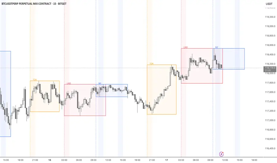
STOCK EXCHANGE + SILVER BULLET FRAMESThis script is an updated version of the " NY/LDN/TOK Stock Exchange Opening Hours " script.
Objective
Displays global stock exchange sessions (New York, London, Tokyo) with session frames, highs/lows, and opening lines. Includes ICT Silver Bullet windows (NY, London, Tokyo) with configurable shading. Past sessions are frozen at close, ongoing sessions update dynamically until closure, and upcoming sessions are pre-drawn. Fully customizable with options for weekends, labels, padding, opacity, and individual session toggles.
It is designed to help traders quickly interpret market context, liquidity zones, and session-based price behavior.
Main Features
Past sessions (historical data)
• Session Frames:
• Each box is frozen at the session’s close.
• The left edge aligns with the opening time, while the right edge is fixed at the closing time.
• The top and bottom reflect the highest and lowest prices during the session.
• Session Labels:
• Names (NY, LDN, TOK) displayed above the frame, aligned left, in the same color as the frame.
• Opening Lines:
• Vertical dotted lines mark the start of each session.
Ongoing and upcoming sessions (live market)
• Dynamic Session Frames:
• The right edge is locked at the future close time.
• The top and bottom update in real time as new highs and lows form.
• Labels and Lines:
• The session label is visible above the active frame.
• Opening lines are drawn as soon as the session begins.
Silver Bullet Time Windows (ICT concept)
• Highlights key liquidity windows within sessions:
• New York: 10:00–11:00 and 14:00–15:00
• London: 08:00–09:00
• Tokyo: 09:00–10:00
• Silver Bullet zones are shaded with configurable opacity (default 5%).
Customization and Options
• Enable or disable individual sessions (NY, London, Tokyo).
• Toggle weekend display (frames and Silver Bullets).
• Adjust label size, padding, and text visibility.
• Control frame opacity (default 0%).
• Optimized memory management with automatic pruning of old graphical objects.
חפש סקריפטים עבור "a股板块+沪深两市+股价不超过10元的股票+技术形态好"
MACROFLOW 200 — Bias & Triggersstephtradez model
MACROFLOW 200 — at a glance (the elevator pitch)
Trade direction = Macro Bias + 1H 200 EMA filter + DXY confirm.
Locations = 1H supply/demand zones.
Triggers (15m): (T1) Retest rejection, (T2) Liquidity sweep + BOS/CHOCH, (T3) Momentum break + shallow pullback.
Stops: structure‑based beyond zone with ATR buffer.
Targets: 2R base, scale at 1.5R, trail to next HTF zone.
Sessions: 7–10 pm ET and 9:30–10:30 am ET.
Risk: tight, prop‑friendly max 1% per session

Body & Volume-Based Buy/Sell Signals (5min 1.5M Vol)Only for 5 min and Volume 1.5M
Conditions (Summarized)
🔹 BUY Signal
Previous candle is red: close < open
Current candle is green: close > open
Previous candle body is smaller than current:
abs(close - open ) < abs(close - open)
Previous candle body size ≥ 10 points
Both candles' volume ≥ minVolume (default: 2,000,000)
➜ Plot BUY below green candle
🔸 SELL Signal
Previous candle is green: close > open
Current candle is red: close < open
Previous candle body is smaller than current:
abs(close - open ) < abs(close - open)
Previous candle body size ≥ 10 points
Both candles' volume ≥ minVolume
➜ Plot SELL above red candle

Multi Volume Weighted Average Price1. Three independent VWAP configurations (VWAP 1, 2, and 3). Each can be set up separately
for periods such as: session, daily, weekly, monthly, etc.
2. Previous VWAP closing prices: Closed VWAPs from previous periods remain visible until the
price touches them. At that point, they are removed.
3. Bands: Based on standard deviation or a percentage of VWAP with an adjustable multiplier.
The bands can be turned on or off.
4. Source: OHLC4 is the default setting for an accurate approximation, but it is customizable
(e.g. HLC3).
5. Global Setting: Select 10,000 or 20,000 historical bars to prevent runtime errors for long
periods.
Usage tips:
1. Use VWAP 1 for daily sessions, VWAP 2 for weekly, and VWAP 3 for Monthly analysis to receive
multi-timeframe support.
2. Customize the labels to clearly distinguish them (e.g. D VWAP, W VWAP, M VWAP).
3. If you encounter errors with historical data (e.g. on the M1 chart), minimize the number of
historical bars displayed to 10,000.

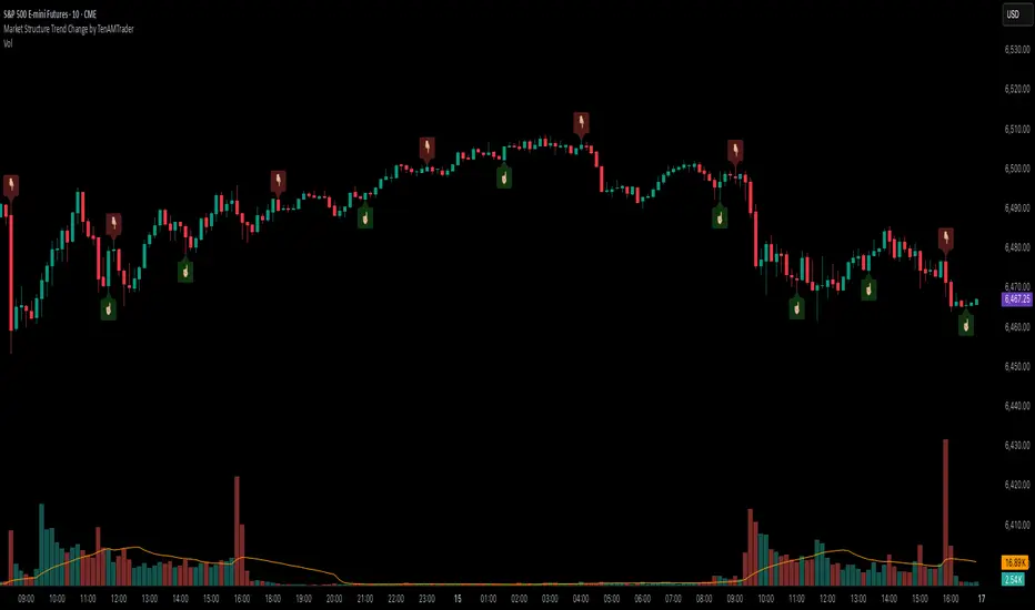
Market Structure Trend Change by TenAMTraderMarket Structure Trend Change Indicator
Description:
This indicator detects changes in market trend by analyzing swing highs and lows to identify Higher Highs (HH), Higher Lows (HL), Lower Highs (LH), and Lower Lows (LL). It helps traders quickly see potential reversals and trend continuation points.
Features:
Automatically identifies pivots based on configurable left and right bars.
Labels pivot points (HH, HL, LH, LL) directly on the chart (text-only for clarity).
Generates buy and sell signals when a trend change is detected:
Buy Signal: HL after repeated LLs.
Sell Signal: LH after repeated HHs.
Fully customizable signal appearance: arrow type, circle, label, color, and size.
Adjustable minimum number of repeated highs or lows before a trend change triggers a signal.
Alerts built in for automated notifications when buy/sell signals occur.
Default Settings:
Optimized for a 10-minute chart.
Default “Min repeats before trend change” and pivot left/right bars are set for typical 10-min price swings.
User Customization:
Adjust the “Pivot Left Bars,” “Pivot Right Bars,” and “Min repeats before trend change” to match your trading style, chart timeframe, and volatility.
Enable pivot labels for visual clarity if desired.
Set alerts to receive notifications of trend changes in real time.
How to Use:
Apply the indicator to any chart and timeframe. It works best on swing-trading or trend-following strategies.
Watch for Buy/Sell signals in conjunction with your other analysis, such as volume, support/resistance, or other indicators.
Legal Disclaimer:
This indicator is provided for educational and informational purposes only. It is not financial advice. Trading involves substantial risk, and past performance is not indicative of future results. Users should trade at their own risk and are solely responsible for any gains or losses incurred.
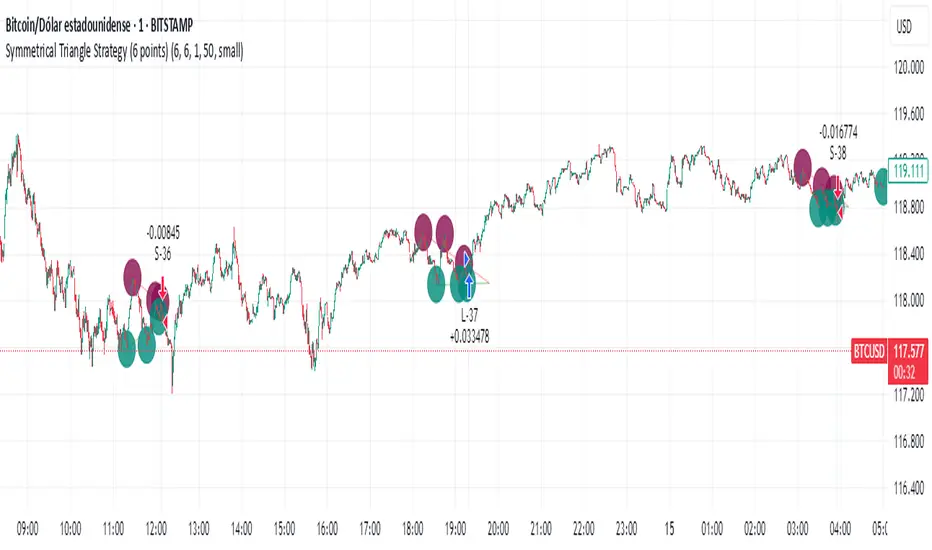
Simple Symmetrical Triangle Strategy (6 points)Overview
This strategy identifies triangle patterns formed by a series of key high and low price points. A trade is triggered when the price breaks out from the pattern's final confirmation points: a buy signal occurs on a close above the last high point, and a sell signal on a close below the last low point. To ensure relevance, any pattern that doesn't break out within 10 bars is automatically discarded.
This helps filter out patterns that lose momentum and focuses only on the most imminent breakouts.
How It Works
1. Pattern Detection: The script continuously scans for a sequence of three declining highs (points H1, H2, H3) and three rising lows (points L1, L2, L3) to form a triangle.
2. Entry Logic: The logic is straightforward and based on breaking the last confirmed pivot:
* Long Entry: A buy order is executed if the price closes above the level of the last high (H3).
* Short Entry: A sell order is executed if the price closes below the level of the last low (L3).
3. Pattern Expiration: A triangle only remains "active" for 10 bars after its formation. If a breakout doesn't occur within this window, the pattern is removed from analysis, avoiding trades on prolonged, unresolved consolidations.
Key Features
* Automatic Detection: Identifies and draws triangles for you.
* Simple Breakout Logic: Easy to understand, trades by following the price action.
* Time Filter: Its main advantage is discarding patterns that do not resolve quickly.
* Customizable: You can adjust the sensitivity of the pivot detection in the settings.
Important Disclaimer
This strategy is designed as an entry system and DOES NOT INCLUDE A STOP LOSS OR TAKE PROFIT.
Automation Ready
Want to automate this or ANY strategy on your broker or MetaTrader (MT4/MT5) without keeping your computer on or needing a VPS? You can use WebhookTrade.
Seasonality Monte Carlo Forecaster [BackQuant]Seasonality Monte Carlo Forecaster
Plain-English overview
This tool projects a cone of plausible future prices by combining two ideas that traders already use intuitively: seasonality and uncertainty. It watches how your market typically behaves around this calendar date, turns that seasonal tendency into a small daily “drift,” then runs many randomized price paths forward to estimate where price could land tomorrow, next week, or a month from now. The result is a probability cone with a clear expected path, plus optional overlays that show how past years tended to move from this point on the calendar. It is a planning tool, not a crystal ball: the goal is to quantify ranges and odds so you can size, place stops, set targets, and time entries with more realism.
What Monte Carlo is and why quants rely on it
• Definition . Monte Carlo simulation is a way to answer “what might happen next?” when there is randomness in the system. Instead of producing a single forecast, it generates thousands of alternate futures by repeatedly sampling random shocks and adding them to a model of how prices evolve.
• Why it is used . Markets are noisy. A single point forecast hides risk. Monte Carlo gives a distribution of outcomes so you can reason in probabilities: the median path, the 68% band, the 95% band, tail risks, and the chance of hitting a specific level within a horizon.
• Core strengths in quant finance .
– Path-dependent questions : “What is the probability we touch a stop before a target?” “What is the expected drawdown on the way to my objective?”
– Pricing and risk : Useful for path-dependent options, Value-at-Risk (VaR), expected shortfall (CVaR), stress paths, and scenario analysis when closed-form formulas are unrealistic.
– Planning under uncertainty : Portfolio construction and rebalancing rules can be tested against a cloud of plausible futures rather than a single guess.
• Why it fits trading workflows . It turns gut feel like “seasonality is supportive here” into quantitative ranges: “median path suggests +X% with a 68% band of ±Y%; stop at Z has only ~16% odds of being tagged in N days.”
How this indicator builds its probability cone
1) Seasonal pattern discovery
The script builds two day-of-year maps as new data arrives:
• A return map where each calendar day stores an exponentially smoothed average of that day’s log return (yesterday→today). The smoothing (90% old, 10% new) behaves like an EWMA, letting older seasons matter while adapting to new information.
• A volatility map that tracks the typical absolute return for the same calendar day.
It calculates the day-of-year carefully (with leap-year adjustment) and indexes into a 365-slot seasonal array so “March 18” is compared with past March 18ths. This becomes the seasonal bias that gently nudges simulations up or down on each forecast day.
2) Choice of randomness engine
You can pick how the future shocks are generated:
• Daily mode uses a Gaussian draw with the seasonal bias as the mean and a volatility that comes from realized returns, scaled down to avoid over-fitting. It relies on the Box–Muller transform internally to turn two uniform random numbers into one normal shock.
• Weekly mode uses bootstrap sampling from the seasonal return history (resampling actual historical daily drifts and then blending in a fraction of the seasonal bias). Bootstrapping is robust when the empirical distribution has asymmetry or fatter tails than a normal distribution.
Both modes seed their random draws deterministically per path and day, which makes plots reproducible bar-to-bar and avoids flickering bands.
3) Volatility scaling to current conditions
Markets do not always live in average volatility. The engine computes a simple volatility factor from ATR(20)/price and scales the simulated shocks up or down within sensible bounds (clamped between 0.5× and 2.0×). When the current regime is quiet, the cone narrows; when ranges expand, the cone widens. This prevents the classic mistake of projecting calm markets into a storm or vice versa.
4) Many futures, summarized by percentiles
The model generates a matrix of price paths (capped at 100 runs for performance inside TradingView), each path stepping forward for your selected horizon. For each forecast day it sorts the simulated prices and pulls key percentiles:
• 5th and 95th → approximate 95% band (outer cone).
• 16th and 84th → approximate 68% band (inner cone).
• 50th → the median or “expected path.”
These are drawn as polylines so you can immediately see central tendency and dispersion.
5) A historical overlay (optional)
Turn on the overlay to sketch a dotted path of what a purely seasonal projection would look like for the next ~30 days using only the return map, no randomness. This is not a forecast; it is a visual reminder of the seasonal drift you are biasing toward.
Inputs you control and how to think about them
Monte Carlo Simulation
• Price Series for Calculation . The source series, typically close.
• Enable Probability Forecasts . Master switch for simulation and drawing.
• Simulation Iterations . Requested number of paths to run. Internally capped at 100 to protect performance, which is generally enough to estimate the percentiles for a trading chart. If you need ultra-smooth bands, shorten the horizon.
• Forecast Days Ahead . The length of the cone. Longer horizons dilute seasonal signal and widen uncertainty.
• Probability Bands . Draw all bands, just 95%, just 68%, or a custom level (display logic remains 68/95 internally; the custom number is for labeling and color choice).
• Pattern Resolution . Daily leans on day-of-year effects like “turn-of-month” or holiday patterns. Weekly biases toward day-of-week tendencies and bootstraps from history.
• Volatility Scaling . On by default so the cone respects today’s range context.
Plotting & UI
• Probability Cone . Plots the outer and inner percentile envelopes.
• Expected Path . Plots the median line through the cone.
• Historical Overlay . Dotted seasonal-only projection for context.
• Band Transparency/Colors . Customize primary (outer) and secondary (inner) band colors and the mean path color. Use higher transparency for cleaner charts.
What appears on your chart
• A cone starting at the most recent bar, fanning outward. The outer lines are the ~95% band; the inner lines are the ~68% band.
• A median path (default blue) running through the center of the cone.
• An info panel on the final historical bar that summarizes simulation count, forecast days, number of seasonal patterns learned, the current day-of-year, expected percentage return to the median, and the approximate 95% half-range in percent.
• Optional historical seasonal path drawn as dotted segments for the next 30 bars.
How to use it in trading
1) Position sizing and stop logic
The cone translates “volatility plus seasonality” into distances.
• Put stops outside the inner band if you want only ~16% odds of a stop-out due to noise before your thesis can play.
• Size positions so that a test of the inner band is survivable and a test of the outer band is rare but acceptable.
• If your target sits inside the 68% band at your horizon, the payoff is likely modest; outside the 68% but inside the 95% can justify “one-good-push” trades; beyond the 95% band is a low-probability flyer—consider scaling plans or optionality.
2) Entry timing with seasonal bias
When the median path slopes up from this calendar date and the cone is relatively narrow, a pullback toward the lower inner band can be a high-quality entry with a tight invalidation. If the median slopes down, fade rallies toward the upper band or step aside if it clashes with your system.
3) Target selection
Project your time horizon to N bars ahead, then pick targets around the median or the opposite inner band depending on your style. You can also anchor dynamic take-profits to the moving median as new bars arrive.
4) Scenario planning & “what-ifs”
Before events, glance at the cone: if the 95% band already spans a huge range, trade smaller, expect whips, and avoid placing stops at obvious band edges. If the cone is unusually tight, consider breakout tactics and be ready to add if volatility expands beyond the inner band with follow-through.
5) Options and vol tactics
• When the cone is tight : Prefer long gamma structures (debit spreads) only if you expect a regime shift; otherwise premium selling may dominate.
• When the cone is wide : Debit structures benefit from range; credit spreads need wider wings or smaller size. Align with your separate IV metrics.
Reading the probability cone like a pro
• Cone slope = seasonal drift. Upward slope means the calendar has historically favored positive drift from this date, downward slope the opposite.
• Cone width = regime volatility. A widening fan tells you that uncertainty grows fast; a narrow cone says the market typically stays contained.
• Mean vs. price gap . If spot trades well above the median path and the upper band, mean-reversion risk is high. If spot presses the lower inner band in an up-sloping cone, you are in the “buy fear” zone.
• Touches and pierces . Touching the inner band is common noise; piercing it with momentum signals potential regime change; the outer band should be rare and often brings snap-backs unless there is a structural catalyst.
Methodological notes (what the code actually does)
• Log returns are used for additivity and better statistical behavior: sim_ret is applied via exp(sim_ret) to evolve price.
• Seasonal arrays are updated online with EWMA (90/10) so the model keeps learning as each bar arrives.
• Leap years are handled; indexing still normalizes into a 365-slot map so the seasonal pattern remains stable.
• Gaussian engine (Daily mode) centers shocks on the seasonal bias with a conservative standard deviation.
• Bootstrap engine (Weekly mode) resamples from observed seasonal returns and adds a fraction of the bias, which captures skew and fat tails better.
• Volatility adjustment multiplies each daily shock by a factor derived from ATR(20)/price, clamped between 0.5 and 2.0 to avoid extreme cones.
• Performance guardrails : simulations are capped at 100 paths; the probability cone uses polylines (no heavy fills) and only draws on the last confirmed bar to keep charts responsive.
• Prerequisite data : at least ~30 seasonal entries are required before the model will draw a cone; otherwise it waits for more history.
Strengths and limitations
• Strengths :
– Probabilistic thinking replaces single-point guessing.
– Seasonality adds a small but meaningful directional bias that many markets exhibit.
– Volatility scaling adapts to the current regime so the cone stays realistic.
• Limitations :
– Seasonality can break around structural changes, policy shifts, or one-off events.
– The number of paths is performance-limited; percentile estimates are good for trading, not for academic precision.
– The model assumes tomorrow’s randomness resembles recent randomness; if regime shifts violently, the cone will lag until the EWMA adapts.
– Holidays and missing sessions can thin the seasonal sample for some assets; be cautious with very short histories.
Tuning guide
• Horizon : 10–20 bars for tactical trades; 30+ for swing planning when you care more about broad ranges than precise targets.
• Iterations : The default 100 is enough for stable 5/16/50/84/95 percentiles. If you crave smoother lines, shorten the horizon or run on higher timeframes.
• Daily vs. Weekly : Daily for equities and crypto where month-end and turn-of-month effects matter; Weekly for futures and FX where day-of-week behavior is strong.
• Volatility scaling : Keep it on. Turn off only when you intentionally want a “pure seasonality” cone unaffected by current turbulence.
Workflow examples
• Swing continuation : Cone slopes up, price pulls into the lower inner band, your system fires. Enter near the band, stop just outside the outer line for the next 3–5 bars, target near the median or the opposite inner band.
• Fade extremes : Cone is flat or down, price gaps to the upper outer band on news, then stalls. Favor mean-reversion toward the median, size small if volatility scaling is elevated.
• Event play : Before CPI or earnings on a proxy index, check cone width. If the inner band is already wide, cut size or prefer options structures that benefit from range.
Good habits
• Pair the cone with your entry engine (breakout, pullback, order flow). Let Monte Carlo do range math; let your system do signal quality.
• Do not anchor blindly to the median; recalc after each bar. When the cone’s slope flips or width jumps, the plan should adapt.
• Validate seasonality for your symbol and timeframe; not every market has strong calendar effects.
Summary
The Seasonality Monte Carlo Forecaster wraps institutional risk planning into a single overlay: a data-driven seasonal drift, realistic volatility scaling, and a probabilistic cone that answers “where could we be, with what odds?” within your trading horizon. Use it to place stops where randomness is less likely to take you out, to set targets aligned with realistic travel, and to size positions with confidence born from distributions rather than hunches. It will not predict the future, but it will keep your decisions anchored to probabilities—the language markets actually speak.

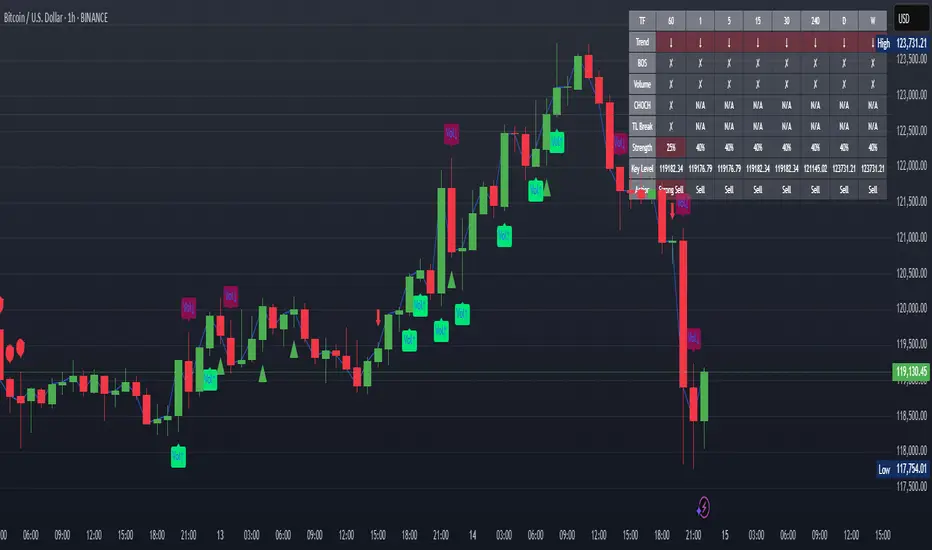
XAUUSD Strength Dashboard with VolumeXAUUSD Strength Dashboard with Volume Analysis
📌 Description
This advanced Pine Script indicator provides a multi-timeframe dashboard for XAUUSD (Gold vs. USD), combining price action analysis with volume confirmation to generate high-probability trading signals. It detects:
✅ Break of Structure (BOS)
✅ Fair Value Gaps (FVG)
✅ Change of Character (CHOCH)
✅ Trendline Breaks (9/21 SMA Crossover)
✅ Volume Spikes (Confirmation of Strength)
The dashboard displays strength scores (0-100%) and action recommendations (Strong Buy/Buy/Neutral/Sell/Strong Sell) across multiple timeframes, helping traders identify confluences for better trade decisions.
🎯 How It Works
1. Multi-Timeframe Analysis
Fetches data from 1m, 5m, 15m, 30m, 1h, 4h, Daily, and Weekly timeframes.
Compares trend direction, BOS, FVG, CHOCH, and volume spikes across all timeframes.
2. Volume-Confirmed Strength Score
The Strength Score (0-100%) is calculated using:
Trend Direction (25 points) → 9 SMA vs. 21 SMA
Break of Structure (20 points) → New highs/lows with momentum
Fair Value Gaps (10 points) → Imbalance zones
Change of Character (10 points) → Shift in market structure
Trendline Break (20 points) → SMA crossover confirmation
Volume Spike (15 points) → High volume confirms moves
Score Interpretation:
≥75% → Strong Buy (High confidence bullish move)
60-74% → Buy (Bullish but weaker confirmation)
40-59% → Neutral (No strong bias)
25-39% → Sell (Bearish but weaker confirmation)
≤25% → Strong Sell (High confidence bearish move)
3. Dashboard & Chart Markers
Dashboard Table: Shows Trend, BOS, Volume, CHOCH, TL Break, Strength %, Key Level, and Action for each timeframe.
Chart Markers:
🟢 Green Triangles → Bullish BOS
🔴 Red Triangles → Bearish BOS
🟢 Green Circles → Bullish CHOCH
🔴 Red Circles → Bearish CHOCH
📈 Green Arrows → Bullish Trendline Break
📉 Red Arrows → Bearish Trendline Break
"Vol↑" (Lime) → Bullish Volume Spike
"Vol↓" (Maroon) → Bearish Volume Spike
🚀 How to Use
1. Dashboard Interpretation
Higher Timeframes (D/W) → Show the dominant trend.
Lower Timeframes (1m-4h) → Help with entry timing.
Strength Score ≥75% or ≤25% → Look for high-confidence trades.
Volume Spikes → Confirm breakouts/reversals.
2. Trading Strategy
📈 Long (Buy) Setup:
Higher TFs (D/W/4h) show bullish trend (↑).
Current TF has BOS & Volume Spike.
Strength Score ≥60%.
Key Level (Low) holds as support.
📉 Short (Sell) Setup:
Higher TFs (D/W/4h) show bearish trend (↓).
Current TF has BOS & Volume Spike.
Strength Score ≤40%.
Key Level (High) holds as resistance.
3. Customization
Adjust Volume Spike Multiplier (Default: 1.5x) → Controls sensitivity to volume spikes.
Toggle Timeframes → Enable/disable higher/lower timeframes.
🔑 Key Benefits
✔ Multi-Timeframe Confluence → Avoids false signals.
✔ Volume Confirmation → Filters low-quality breakouts.
✔ Clear Strength Scoring → Removes emotional bias.
✔ Visual Chart Markers → Easy to spot key signals.
This indicator is ideal for gold traders who follow institutional order flow, market structure, and volume analysis to improve their trading decisions.
🎯 Best Used With:
Support/Resistance Levels
Fibonacci Retracements
Price Action Confirmation
🚀 Happy Trading! 🚀
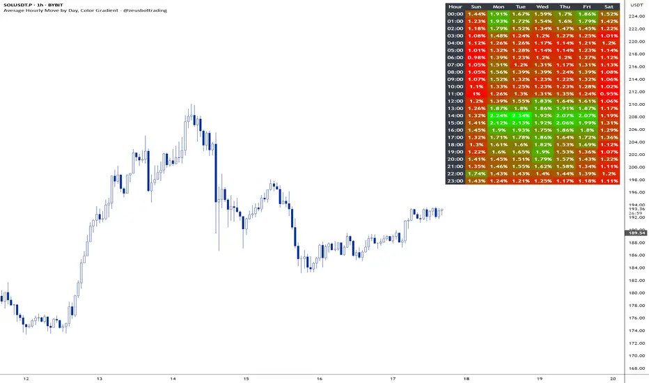
Average hourly move by @zeusbottradingThis Pine Script called "Average hourly move by @zeusbottrading" calculates and displays the average percentage price movement for each hour of the day using the full available historical data.
How the script works:
It tracks the high and low price within each full hour (e.g., 10:00–10:59).
It calculates the percentage move as the range between high and low relative to the average price during that hour.
For each hour of the day, it stores the total of all recorded moves and the count of occurrences across the full history.
At the end, the script computes the average move for each hour (0 to 23) and determines the minimum and maximum averages.
Using these values, it creates a color gradient, where the hours with the lowest average volatility are red and the highest are green.
It then displays a table in the top-right corner of the chart showing each hour and its average percentage move, color‑coded according to volatility.
What it can be used for:
Identifying when the market is historically most volatile or calm during the day.
Helping plan trade entries and exits based on expected volatility.
Comparing hourly volatility patterns across different markets or instruments.
Adjusting position size and risk management according to the anticipated volatility in a particular hour.
Using long-term historical data to understand recurring daily volatility patterns.
In short, this script is a useful tool for traders who want to fine‑tune their trading strategies and risk management by analyzing time‑based volatility profiles.
Prime NumbersPrime Numbers highlights prime numbers (no surprise there 😅), tokens and the recent "active" feature in "input".
🔸 CONCEPTS
🔹 What are Prime Numbers?
A prime number (or a prime) is a natural number greater than 1 that is not a product of two smaller natural numbers.
Wikipedia: Prime number
🔹 Prime Factorization
The fundamental theorem of arithmetic states that every integer larger than 1 can be written as a product of one or more primes. More strongly, this product is unique in the sense that any two prime factorizations of the same number will have the same number of copies of the same primes, although their ordering may differ. So, although there are many different ways of finding a factorization using an integer factorization algorithm, they all must produce the same result. Primes can thus be considered the "basic building blocks" of the natural numbers.
Wikipedia: Fundamental theorem of arithmetic
Math Is Fun: Prime Factorization
We divide a given number by Prime Numbers until only Primes remain.
Example:
24 / 2 = 12 | 24 / 3 = 8
12 / 3 = 4 | 8 / 2 = 4
4 / 2 = 2 | 4 / 2 = 2
|
24 = 2 x 3 x 2 | 24 = 3 x 2 x 2
or | or
24 = 2² x 3 | 24 = 2² x 3
In other words, every natural/integer number above 1 has a unique representation as a product of prime numbers, no matter how the number is divided. Only the order can change, but the factors (the basic elements) are always the same.
🔸 USAGE
The Prime Numbers publication contains two use cases:
Prime Factorization: performed on "close" prices, or a manual chosen number.
List Prime Numbers: shows a list of Prime Numbers.
The other two options are discussed in the DETAILS chapter:
Prime Factorization Without Arrays
Find Prime Numbers
🔹 Prime Factorization
Users can choose to perform Prime Factorization on close prices or a manually given number.
❗️ Note that this option only applies to close prices above 1, which are also rounded since Prime Factorization can only be performed on natural (integer) numbers above 1.
In the image below, the left example shows Prime Factorization performed on each close price for the latest 50 bars (which is set with "Run script only on 'Last x Bars'" -> 50).
The right example shows Prime Factorization performed on a manually given number, in this case "1,340,011". This is done only on the last bar.
When the "Source" option "close price" is chosen, one can toggle "Also current price", where both the historical and the latest current price are factored. If disabled, only historical prices are factored.
Note that, depending on the chosen options, only applicable settings are available, due to a recent feature, namely the parameter "active" in settings.
Setting the "Source" option to "Manual - Limited" will factorize any given number between 1 and 1,340,011, the latter being the highest value in the available arrays with primes.
Setting to "Manual - Not Limited" enables the user to enter a higher number. If all factors of the manual entered number are in the 1 - 1,340,011 range, these factors will be shown; however, if a factor is higher than 1,340,011, the calculation will stop, after which a warning is shown:
The calculated factors are displayed as a label where identical factors are simplified with an exponent notation in superscript.
For example 2 x 2 x 2 x 5 x 7 x 7 will be noted as 2³ x 5 x 7²
🔹 List Prime Numbers
The "List Prime Numbers" option enables users to enter a number, where the first found Prime Number is shown, together with the next x Prime Numbers ("Amount", max. 200)
The highest shown Prime Number is 1,340,011.
One can set the number of shown columns to customize the displayed numbers ("Max. columns", max. 20).
🔸 DETAILS
The Prime Numbers publication consists out of 4 parts:
Prime Factorization Without Arrays
Prime Factorization
List Prime Numbers
Find Prime Numbers
The usage of "Prime Factorization" and "List Prime Numbers" is explained above.
🔹 Prime Factorization Without Arrays
This option is only there to highlight a hurdle while performing Prime Factorization.
The basic method of Prime Factorization is to divide the base number by 2, 3, ... until the result is an integer number. Continue until the remaining number and its factors are all primes.
The division should be done by primes, but then you need to know which one is a prime.
In practice, one performs a loop from 2 to the base number.
Example:
Base_number = input.int(24)
arr = array.new()
n = Base_number
go = true
while go
for i = 2 to n
if n % i == 0
if n / i == 1
go := false
arr.push(i)
label.new(bar_index, high, str.tostring(arr))
else
arr.push(i)
n /= i
break
Small numbers won't cause issues, but when performing the calculations on, for example, 124,001 and a timeframe of, for example, 1 hour, the script will struggle and finally give a runtime error.
How to solve this?
If we use an array with only primes, we need fewer calculations since if we divide by a non-prime number, we have to divide further until all factors are primes.
I've filled arrays with prime numbers and made libraries of them. (see chapter "Find Prime Numbers" to know how these primes were found).
🔹 Tokens
A hurdle was to fill the libraries with as many prime numbers as possible.
Initially, the maximum token limit of a library was 80K.
Very recently, that limit was lifted to 100K. Kudos to the TradingView developers!
What are tokens?
Tokens are the smallest elements of a program that are meaningful to the compiler. They are also known as the fundamental building blocks of the program.
I have included a code block below the publication code (// - - - Educational (2) - - - ) which, if copied and made to a library, will contain exactly 100K tokens.
Adding more exported functions will throw a "too many tokens" error when saving the library. Subtracting 100K from the shown amount of tokens gives you the amount of used tokens for that particular function.
In that way, one can experiment with the impact of each code addition in terms of tokens.
For example adding the following code in the library:
export a() => a = array.from(1) will result in a 100,041 tokens error, in other words (100,041 - 100,000) that functions contains 41 tokens.
Some more examples, some are straightforward, others are not )
// adding these lines in one of the arrays results in x tokens
, 1 // 2 tokens
, 111, 111, 111 // 12 tokens
, 1111 // 5 tokens
, 111111111 // 10 tokens
, 1111111111111111111 // 20 tokens
, 1234567890123456789 // 20 tokens
, 1111111111111111111 + 1 // 20 tokens
, 1111111111111111111 + 8 // 20 tokens
, 1111111111111111111 + 9 // 20 tokens
, 1111111111111111111 * 1 // 20 tokens
, 1111111111111111111 * 9 // 21 tokens
, 9999999999999999999 // 21 tokens
, 1111111111111111111 * 10 // 21 tokens
, 11111111111111111110 // 21 tokens
//adding these functions to the library results in x tokens
export f() => 1 // 4 tokens
export f() => v = 1 // 4 tokens
export f() => var v = 1 // 4 tokens
export f() => var v = 1, v // 4 tokens
//adding these functions to the library results in x tokens
export a() => const arraya = array.from(1) // 42 tokens
export a() => arraya = array.from(1) // 42 tokens
export a() => a = array.from(1) // 41 tokens
export a() => array.from(1) // 32 tokens
export a() => a = array.new() // 44 tokens
export a() => a = array.new(), a.push(1) // 56 tokens
What if we could lower the amount of tokens, so we can export more Prime Numbers?
Look at this example:
829111, 829121, 829123, 829151, 829159, 829177, 829187, 829193
Eight numbers contain the same number 8291.
If we make a function that removes recurrent values, we get fewer tokens!
829111, 829121, 829123, 829151, 829159, 829177, 829187, 829193
//is transformed to:
829111, 21, 23, 51, 59, 77, 87, 93
The code block below the publication code (// - - - Educational (1) - - - ) shows how these values were reduced. With each step of 100, only the first Prime Number is shown fully.
This function could be enhanced even more to reduce recurrent thousands, tens of thousands, etc.
Using this technique enables us to export more Prime Numbers. The number of necessary libraries was reduced to half or less.
The reduced Prime Numbers are restored using the restoreValues() function, found in the library fikira/Primes_4.
🔹 Find Prime Numbers
This function is merely added to show how I filled arrays with Prime Numbers, which were, in turn, added to libraries (after reduction of recurrent values).
To know whether a number is a Prime Number, we divide the given number by values of the Primes array (Primes 2 -> max. 1,340,011). Once the division results in an integer, where the divisor is smaller than the dividend, the calculation stops since the given number is not a Prime.
When we perform these calculations in a loop, we can check whether a series of numbers is a Prime or not. Each time a number is proven not to be a Prime, the loop starts again with a higher number. Once all Primes of the array are used without the result being an integer, we have found a new Prime Number, which is added to the array.
Doing such calculations on one bar will result in a runtime error.
To solve this, the findPrimeNumbers() function remembers the index of the array. Once a limit has been reached on 1 bar (for example, the number of iterations), calculations will stop on that bar and restart on the next bar.
This spreads the workload over several bars, making it possible to continue these calculations without a runtime error.
The result is placed in log.info() , which can be copied and pasted into a hardcoded array of Prime Number values.
These settings adjust the amount of workload per bar:
Max Size: maximum size of Primes array.
Max Bars Runtime: maximum amount of bars where the function is called.
Max Numbers To Process Per Bar: maximum numbers to check on each bar, whether they are Prime Numbers.
Max Iterations Per Bar: maximum loop calculations per bar.
🔹 The End
❗️ The code and description is written without the help of an LLM, I've only used Grammarly to improve my description (without AI :) )

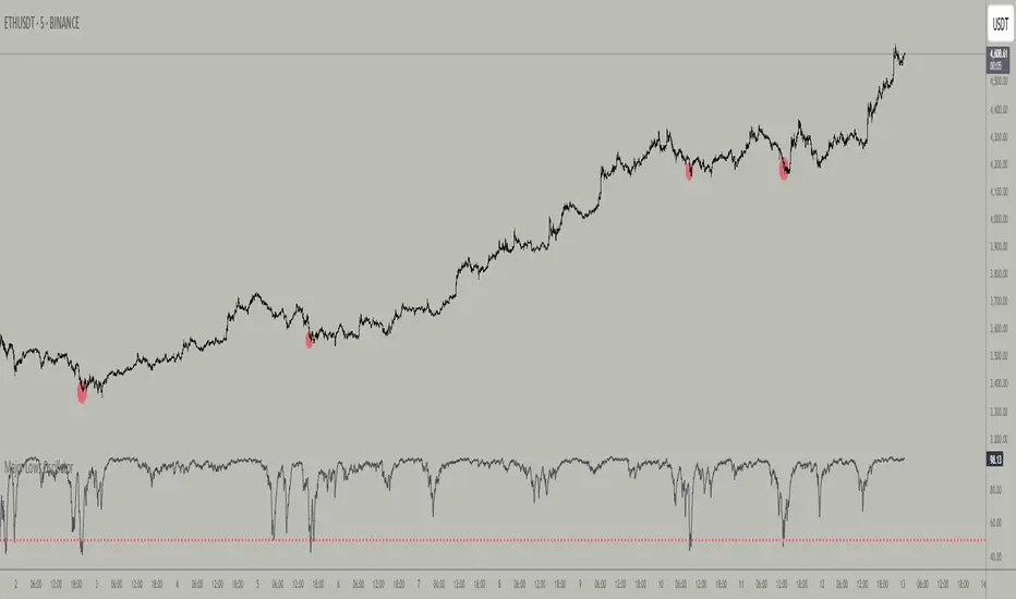
Major Lows OscillatorDescription
The Major Lows Oscillator is a custom technical indicator designed to identify significant low-price areas by normalizing the current closing price relative to recent lowest lows and highest highs. The oscillator calculates a normalized price percentage over a configurable lookback period, applies exponential moving averages for smoothing, and inverts the result to highlight potential market bottoms.
Calculation Details
Lowest Low Lookback : Finds the lowest low over a user-defined period (default 100 bars).
Highest High Lookback : Calculates the highest high over a short period (default 1 bar), providing a dynamic normalization range.
Normalization : Normalizes the current close within the range defined by the lowest low and highest high, scaled to 0-100.
Smoothing : Applies a 10-period EMA, inversion, and weighted smoothing combining the last valid value and current oscillator reading.
Final Output : Applies a final EMA (period 1) and inverts the oscillator (100 - value) to emphasize major lows.
Features
Customizable midline level for signal alerts (default 50).
Visual midline reference line.
Alerts trigger on oscillator crossing below midline for automated monitoring.
Usage
Useful for complementing existing setups or integration in algorithmic trading strategies.
Changing the input parameters opens new ways to leverage the asymmetric range concept, allowing adaptation to different market regimes and enhancing the oscillator’s sensitivity and utility.
Examples of input combinations and their potential purposes include:
Extremely Asymmetric Setting: Lowest Low Lookback = 200, Highest High Lookback = 1
Focuses on deep long-term lows contrasted with immediate highs, ideal for spotting strong oversold levels within an otherwise bullish short-term momentum.
Symmetric Lookbacks: Lowest Low Lookback = Highest High Lookback = 50
Balances the range equally, creating a normalized oscillator that treats recent lows and highs with the same weight — useful for markets with balanced volatility.
Short but Equal Lookbacks: Lowest Low Lookback = Highest High Lookback = 10
Highly sensitive to recent price swings, this setting can detect rapid shifts and is suited for intraday or very short-term trading.
Inverted Extreme: Lowest Low Lookback = 1, Highest High Lookback = 100
Highlights very recent lows against a long-term high range, possibly signaling quick dips in a generally overextended market.
Inputs
Midline Level : Threshold for alerts (default 50).
Lowest Low Lookback Period : Bars evaluated for lowest low (default 100).
Highest High Lookback Period : Bars evaluated for highest high (default 1).
Alerts
Configured to trigger once per bar close when the oscillator crosses below the midline level.
---
Disclaimer
This indicator is for educational and analytical use only.
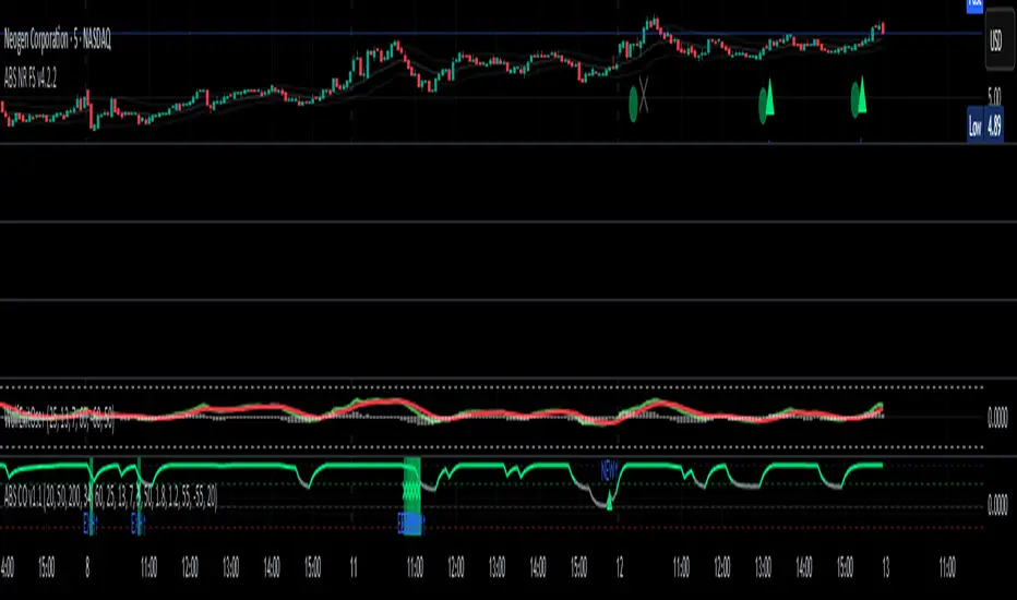
ABS NR — Fail-Safe Confirm (v4.2.2)
# ABS NR — Fail-Safe Confirm (v4.2.2)
## What it is (quick take)
**ABS NR FS** is a **non-repainting “arm → confirm” entry framework** for intraday and swing execution. It blends:
* **Regime** (EMA stack + 60-min slope),
* **Location** (Keltner basis/edges),
* **Stretch** (session-anchored **VWAP Z-score**),
* **Momentum gating** (TSI cross/slope),
* **Guards** (session window, minimum ATR%, gap filter, optional market alignment).
You’ll see a **small dot** when a setup is **armed** (candidate) and a **triangle** when that setup **confirms** within a user-defined number of bars. A **gray “X”** marks a timeout (candidate canceled).
> Tip: This entry tool works best when paired with a trend context filter and a dedicated exit tool.
---
## How to use it (operational workflow)
1. **Read the regime**
* **Bull trend**: fast > slow > long EMA **and** 60-min slope up.
* **Bear trend**: fast < slow < long EMA **and** 60-min slope down.
* **Range**: neither bull nor bear.
2. **Wait for a candidate (dot)**
Two families:
* **Reclaim (trend-following):** price crosses the **KC basis** with acceptable |Z| (not overstretched) and passes the TSI gate.
* **Fade (range-revert):** price **pokes a KC band**, prints a **reversal wick**, |Z| is stretched, and TSI gate agrees.
3. **Trade the confirmation (triangle)**
The confirm must occur **within N bars** and follow your chosen **Confirm mode** logic (see Inputs). If confirmation doesn’t arrive in time, an **X** cancels the candidate.
4. **Use guards to avoid junk**
Session windows (US focus), minimum ATR%, gap guard, and optional **market alignment** (e.g., SPY above EMA20 for longs).
5. **Manage the position**
* Entries: take **triangles** in the direction of your playbook (reclaims with trend; fades in clean ranges).
* Filters and exits: use your own process or pair with a trend/exit companion.
---
## Visual semantics & alerts
* **Candidate L / S (dot)** → a setup armed on this bar.
* **CONFIRM L / S (triangle)** → actionable signal that met confirm rules within your time window.
* **Cancel L / S (X)** → candidate expired without confirmation; ignore the dot.
**Alerts (stable names for automation):**
* **ABS FS — Confirmed** → fires on confirmed long or short.
* **ABS FS — Candidate Armed** → fires as a candidate arms.
---
## Non-repainting behavior (why signals don’t repaint)
* All HTF requests use **lookahead\_off**.
* With **Strict NR = true**, the 60-min slope uses the **prior completed** 60-min bar and arming/confirming only occurs on confirmed bars.
* Confirmation triangles finalize on bar close.
* If you disable strictness, signals may appear slightly earlier but with more intrabar sensitivity.
---
## Inputs reference (what each control does and the trade-offs)
### A) Behavior / Modes
**Mode** (`Turbo / Aggressive / Balanced / Conservative`)
Changes multiple internal thresholds:
* **Turbo** → most signals; relaxes prior-bar break & VWAP-side checks and time/vol/gap guards. Highest frequency, highest noise.
* **Aggressive** → more signals than Balanced, fewer than Turbo.
* **Balanced** → default; steady trade-off of frequency vs. quality.
* **Conservative** → tightens |Z| and other checks; fewest but cleanest signals.
**Strict NR (bar close + prior HTF 60m)**
* **true** = safer: uses prior 60-min slope; arms/confirms on confirmed bars → **fewer/cleaner** signals.
* **false** = earlier and more reactive; slightly noisier.
---
### B) Keltner Channel (location engine)
* **KC EMA Length (`kcLen`)**
Higher → smoother basis (fewer basis crosses). Lower → snappier basis (more crosses).
* **ATR Length (`atrLen`)**
Higher → steadier band width; Lower → more reactive band width.
* **KC ATR Mult (`kcMult`)**
Higher → wider bands (fewer edge pokes → fewer fades). Lower → narrower (more fades).
---
### C) Trend & HTF slope
* **Trend EMA Fast/Slow/Long (`emaFastLen / emaSlowLen / emaLongLen`)**
Larger = slower regime flips (fewer reclaims); smaller = faster flips (more reclaims).
* **HTF EMA Len (60m) (`htfLen`)**
Larger = steadier HTF slope (fewer signals); smaller = more sensitive (more signals).
---
### D) VWAP Z-Score (stretch / mean-revert logic)
* **VWAP Z-Length (`zLen`)**
Window for Z over session-anchored VWAP distance. Larger = smoother |Z| (fewer fades/re-entries). Smaller = more reactive (more).
* **Range Fade |Z| (base) (`zFadeBase`)**
Minimum |Z| to allow **fades** in ranges. Raise to demand more stretch (fewer fades). Lower to take more fades.
* **Max |Z| Trend Re-entry (base) (`maxZTrendBase`)**
Caps how stretched price can be and still permit **reclaims** with trend. Lower = stricter (avoid chases). Higher = will chase further.
---
### E) TSI Momentum Gate
* **TSI Long/Short/Signal (`tsiLong / tsiShort / tsiSig`)**
Larger = smoother/laggier momentum; smaller = snappier.
* **TSI gate (`CrossOnly / CrossOrSlope / Off`)**
* **CrossOnly**: require TSI cross of its signal (strict).
* **CrossOrSlope**: cross *or* favorable slope (balanced default).
* **Off**: no momentum gate (most signals, most noise).
---
### F) Guards (filters to avoid low-quality tape)
* **US focus 09:35–10:30 & 14:00–15:45 (base) (`useTimeBase`)**
`true` limits to high-quality windows. `false` trades all session.
* **Skip N bars after 09:30 ET (`skipFirst`)**
Skips the open scramble. Larger = skip longer.
* **Min volatility ATR% (base)** = `useVolMinBase` + `atrPctMinBase`
Requires `ATR(10)/Close*100 ≥ atrPctMinBase`. Raise threshold to avoid dead tape; lower to accept quieter sessions.
* **Gap guard (base)** = `gapGuardBase` + `gapMul`
Blocks signals when the opening gap exceeds `gapMul * ATR`. Increase `gapMul` to allow more gapped opens; decrease to be stricter.
---
### G) Visuals & Sides
* **Plot Keltner (`plotKC`)** → show/hide basis & bands.
* **Show Longs / Show Shorts** → enable/disable each side.
---
### H) Fail-Safe Confirmation
* **Confirm mode (`BreakHighOnly / BreakHigh+Hold / TwoBarImpulse`)**
* **BreakHighOnly**: confirm by taking out the armed bar’s extreme. Fastest, most frequent.
* **BreakHigh+Hold**: must **break**, have **body ≥ X·ATR**, **and** hold above/below the basis → higher quality, fewer signals.
* **TwoBarImpulse**: decisive follow-through vs. prior bar with **body ≥ X·ATR** → momentum-biased confirmations.
* **Confirm within N bars (`confirmBars`)**
Confirmation window size. Smaller = faster validation; larger = more patience (can be later).
* **Impulse body ≥ X·ATR (`impulseBodyATR`)**
Raise for stronger confirmations (fewer weak triangles). Lower to accept lighter pushes.
* **Require market alignment (`needMarket`) + `marketTicker`**
When enabled: Longs require **market > EMA20 (5m)**; Shorts require **market < EMA20 (5m)**.
* **Diagnostics: Show debug letters (`debug`)**
Tiny “B/C” audit marks for base/confirm while tuning.
---
## Tuning recipes (quick, practical)
* **If you’re getting chopped:**
* Set **Mode = Conservative**
* **Confirm mode = BreakHigh+Hold**
* Raise **impulseBodyATR** (e.g., 0.45)
* Keep **needMarket = true**
* Keep **Strict NR = true**
* **If you need more signals:**
* **Mode = Aggressive** (or Turbo if you accept more noise)
* **Confirm mode = BreakHighOnly**
* Lower **impulseBodyATR** (0.25–0.30)
* Increase **confirmBars** to 3
* **Range-day focus (fades):**
* Keep session guard on
* Raise **zFadeBase** to demand real stretch
* Keep **maxZTrendBase** moderate (don’t chase)
* **Trend-day focus (reclaims):**
* Slightly **lower `maxZTrendBase`** (avoid chasing excessive stretch)
* Use **CrossOrSlope** TSI gating
* Consider turning **needMarket** on
---
## Best practices & notes
* **Instrument specificity:** Tune Z, TSI, and guards per symbol and timeframe.
* **Session awareness:** Session filter uses **exchange-local** time; adjust for non-US markets.
* **Automation:** Use the two provided alert names; they’re stable.
* **Risk management:** Confirmation improves quality but doesn’t remove risk. Always pre-define stop/size logic.
---
## Suggested starting point (balanced profile)
* **Mode = balanced**
* **Strict NR = true**
* **Confirm mode = BreakHigh+Hold**
* **confirmBars = 2**
* **impulseBodyATR ≈ 0.35**
* **needMarket = off** (turn on for extra confluence)
* Leave Keltner/TSI defaults; then nudge `zFadeBase` and `maxZTrendBase` to match your symbol.
---
*This tool is a signal generator, not a broker or strategy. Validate on your markets/timeframes and integrate with your risk plan.*
Key Indicators Dashboard (KID)Key Indicators Dashboard (KID) — Comprehensive Market & Trend Metrics
📌 Overview
The Key Indicators Dashboard (KID) is an advanced multi-metric market analysis tool designed to consolidate essential technical, volatility, and relative performance data into a single on-chart table. Instead of switching between multiple indicators, KID centralizes these key measures, making it easier to assess a stock’s technical health, volatility state, trend status, and relative strength at a glance.
🛠 Key Features
⦿ Average Daily Range (ADR %): Measures average daily price movement over a specified period. It is calculated by averaging the daily price range (high - low) over a set number of days (default 20 days).
⦿ Average True Range (ATR): Measures volatility by calculating the average of a true range over a specific period (default 14). It helps traders gauge the typical extent of price movement, regardless of the direction.
⦿ ATR%: Expresses the Average True Range as a percentage of the price, which allows traders to compare the volatility of stocks with different prices.
⦿ Relative Strength (RS): Compares a stock’s performance to a chosen benchmark index (default NIFTYMIDSML400) over a specific period (default 50 days).
⦿ RS Score (IBD-style): A normalized 1–100 rating inspired by Investor’s Business Daily methodology.
How it works: The RS Score is based on a weighted average of price changes over 3 months (40%), 6 months (20%), 9 months (20%), and 12 months (20%).
The raw value is converted into a percentage return, then normalized over the past 252 trading days so the lowest value maps to 1 and the highest to 100.
This produces a percentile-style score that highlights the strongest stocks in relative terms.
⦿ Relative Volume (RVol): Compares a stock's current volume to its average volume over a specific period (default 50). It is calculated by dividing the current volume by the average historical volume.
⦿ Average ₹ Volume (Turnover): Represents the total monetary value of shares traded for a stock. It's calculated by multiplying a day's closing price by its volume, with the final value converted to crores for clarity. This metric is a key indicator of a stock's liquidity and overall market interest.
⦿ Moving Average Extension: Measures how far a stock's current price has moved from from a selected moving average (EMA or SMA). This deviation is normalized by the stock's volatility (ATR%), with a default threshold of 6 ATR used to indicate that the stock is significantly extended and is marked with a selected shape (default Red Flag).
⦿ 52-Weeks High & Low: Measures a stock's current price in relation to its highest and lowest prices over the past year. It calculates the percentage a stock is below its 52-week high and above its 52-week low.
⦿ Market Capitalization: Market Cap represents the total value of all outstanding.
⦿ Free Float: It is the value of shares readily available for public trading, with the Free Float Percentage showing the proportion of shares available to the public.
⦿ Trend: Uses Supertrend indicator to identify the current trend of a stock's price. A factor (default 3) and an ATR period (default 10) is used to signal whether the trend is up or down.
⦿ Minervini Trend Template (MTT): It is a set of technical criteria designed to identify stocks in strong uptrends.
Price > 50-DMA > 150-DMA > 200-DMA
200-DMA is trending up for at least 1 month
Price is at least 30% above its 52-week low.
Price is within at least 25 percent of its 52-week high
Table highlights when a stock meets all above criteria.
⦿ Sector & Industry: Display stock's sector and industry, provides categorical classification to assist sector-based analysis. The sector is a broad economic classification, while the industry is a more specific group within that sector.
⦿ Moving Averages (MAs): Plot up to four customizable Moving Averages on a chart. You can independently set the type (Simple or Exponential), the source price, and the length for each MA to help visualize a stock's underlying trend.
MA1: Default 10-EMA
MA2: Default 20-EMA
MA3: Default 50-EMA
MA4: Default 200-EMA
⦿ Moving Average (MA) Crossover: It is a trend signal that occurs when a shorter-term moving average crosses a longer-term one. This script identifies these crossover events and plots a marker on the chart to visually signal a potential change in trend direction.
User-configurable MAs (short and long).
A bullish crossover occurs when the short MA crosses above the long MA.
A bearish crossover occurs when the short MA crosses below the long MA.
⦿ Inside Bar (IB): An Inside Bar is a candlestick whose entire price range is contained within the range of the previous bar. This script identifies this pattern, which often signals consolidation, and visually marks bullish and bearish inside bars on the chart with distinct colors and labels.
⦿ Tightness: Identifies periods of low volatility and price consolidation. It compares the price range over a short lookback period (default 3) to the average daily range (ADR). When the lookback range is smaller than the ADR, the indicator plots a marker on the chart to signal consolidation.
⦿ PowerBar (Purple Dot): Identifies candles with a strong price move on high volume. By default, it plots a purple dot when a stock moves up or down by at least 5% and has a minimum volume of 500,000. More dots indicate higher volatility and liquidity.
⦿ Squeezing Range (SQ): Identifies periods of low volatility, which can often precede a significant price move. It checks if the Bollinger Bands have narrowed to a range that is smaller than the Average True Range (ATR) for a set number of consecutive bars (default 3).
(UpperBB - LowerBB) < (ATR × 2)
⦿ Mark 52-Weeks High and Low: Marks and labels a stock's 52-Week High and Low prices directly on the chart. It draws two horizontal lines extending from the candles where the highest and lowest prices occurred over the past year, providing a clear visual reference for long-term price extremes.
⏳PineScreener Filters
The indicator’s alert conditions act as filters for PineScreener.
Price Filter: Minimum and maximum price cutoffs (default ₹25 - ₹10000).
Daily Price Change Filter: Minimum and maximum daily percent change (default -5% and 5%).
🔔 Built-in Alerts
Supports alert creation for:
ADR%, ATR/ATR %, RS, RS Rating, Turnover
Moving Average Crossover (Bullish/Bearish)
Minervini Trend Template
52-Week High/Low
Inside Bars (Bullish/Bearish)
Tightness
Squeezing Range (SQ)
⚙️ Customizable Visualization
Switchable between vertical or horizontal layout.
Works in dark/light mode
User-configurable to toggle any indicator ON or OFF.
User-configurable Moving (EMA/SMA), Period/Lengths and thresholds.
⦿ (Optional) : For horizontal table orientation increase Top Margin to 16% in Chart (Canvas) settings to avoid chart overlapping with table.
⚡ Add this script to your chart and start making smarter trade decisions today! 🚀

Relative Strength Range RankRelative Strength Range Rank – Chart Asset vs. Benchmarks
Description:
This indicator calculates and ranks the relative strength position of the current chart’s asset against up to five user-defined comparison symbols. By default, the comparison set is USDT.D, USDC.D and DAI.D.
Calculation method:
The same oscillator calculation is applied identically to the current chart’s asset and all comparison symbols:
For each symbol:
Determine the lowest low over LOWEST bars.
Determine the highest high over HIGHEST bars.
Calculate normalized position within range:
raw_osc = (close - lowest_low) / (highest_high - lowest_low) * 100
Apply a 10-period EMA to smooth raw_osc.
Invert and scale to match assets direction:
raw_osc = 100 - EMA_10(raw_osc)
Apply weighted smoothing:
smoothed = 0.191 * previous_value + 0.809 * current_value
Apply a final 1-period EMA to reduce jitter.
Output is the inverted smoothed oscillator value, representing the relative strength rank.
This function is implemented as calculate_oscillator() and used for all input symbols plus the current chart symbol, ensuring consistency in comparative analysis.
Plotting:
Each comparison symbol oscillator is plotted in the indicator pane.
The current chart oscillator is always plotted in black.
Alert condition:
Boolean chart_osc_above_all is true when the current chart oscillator is strictly greater than all other comparison oscillator values.
The alert chart_osc_crossed_above triggers only on the first bar where chart_osc_above_all changes from false to true.
Smoothing advantage:
The smoothing sequence (EMA → weighted smoothing → EMA) is designed to reduce short-term noise while preserving responsiveness to changes in price position.
The initial EMA(10) filters random fluctuations.
The weighted smoothing step (0.191 * prev + 0.809 * current) reduces overshoot and dampens oscillations without introducing significant lag, unlike longer EMAs.
The final EMA(1) step ensures stability in the plotted oscillator without visible jaggedness.
This combination yields a signal that is both smooth and reactive, making relative strength comparisons more precise.
Inputs:
Sym 1–5: up to five comparison tickers.
Lowest low lookback period ( LOWEST ).
Highest high lookback period ( HIGHEST ).
Color for plotted comparison lines.
Output:
Oscillator values from 0 to 100, where higher values indicate that the asset’s current price is closer to the highest high of the lookback period, and lower values indicate proximity to the lowest low.
Sorted table showing all selected assets ranked by oscillator value.
Optional alert when the current chart asset leads all selected assets in oscillator value.
Short Description:
Computes range-normalized oscillator values for the chart asset and up to 5 symbols, using EMA and weighted smoothing to reduce noise while preserving responsiveness; optional alert when the chart asset exceeds all others.

RSI Momentum Divergence Zones [ChartPrime]⯁ OVERVIEW
RSI Momentum Divergence Zones is a hybrid oscillator and chart overlay tool that detects RSI-based momentum divergences and projects them as key zones on the chart. By combining RSI divergence logic with horizontal level plotting, this indicator reveals high-probability support and resistance areas where price has historically reacted to hidden or classic divergences.
⯁ KEY FEATURES
Momentum-Based RSI Source:
Instead of the classic RSI input, this tool uses the momentum of price as the RSI source:
rsiSrc = ta.mom(close, 10)
This emphasizes acceleration and deceleration of price moves, sharpening divergence signals and making them more responsive to early shifts in momentum.
Automatic Divergence Detection (Optional):
When enabled, the indicator continuously scans for:
— Bullish Divergence : Price makes a Lower Low while RSI forms a Higher Low
— Bearish Divergence : Price makes a Higher High while RSI forms a Lower High
It ensures divergence is valid by checking the spacing between pivots (min 5, max 50 bars).
Divergence Labels & Markers (RSI Pane + Chart):
When a valid divergence is detected:
— On RSI pane:
Labels appear at HL/LH points (“Bull” / “Bear”)
Colored lines show pivot structures
— On price chart:
Labels (“▲ Bull” / “Bear ▼”) mark price pivot that triggered the divergence
Lines highlight the exact price level at the divergence origin
Divergence Zones / Levels (Toggleable):
The indicator projects horizontal zones across the chart based on confirmed divergence points.
These levels dynamically extend as long as price respects them, and auto-expire once broken.
They act as S/R levels created by market imbalance caused by divergence reactions.
Dynamic Zone Extension Logic:
Once plotted, divergence levels will extend to the right:
— If price respects the level, the zone keeps growing
— If broken in the opposite direction, the level stops extending and turns dashed (visually showing break)
Zone Layering and Limit Control:
You can limit the number of simultaneous zones shown on the chart (e.g., 10 most recent).
Old zones automatically expire and are removed to keep the chart clean and focused.
Color Customization and Intensity:
Different colors for bullish and bearish zones let you easily distinguish trend direction.
Background fill, line width, and transparency are all adjustable.
Clean Zone Management with Arrays:
Behind the scenes, the script uses custom divLevel type arrays to manage plotted levels, ensuring they stay up-to-date, extend correctly, and delete once invalidated.
⯁ USAGE
Use bullish divergence zones as potential demand areas and bearish ones as supply zones.
Combine RSI pane labels with price-level zones to confirm strength of reversal.
Watch for price approaching a divergence level to anticipate reactions or breakouts.
Use divergence levels as trade triggers, stop-loss guides, or take-profit markers.
Limit signal count using the “Qty Divergence Zones” setting to reduce chart clutter.
Enable divergence detection only when you want to focus on key structural zones — ideal for swing or positional setups.
⯁ CONCLUSION
RSI Momentum Divergence Zones blends oscillator divergence logic with price action structure to uncover hidden strength or weakness in the market. With flexible zone plotting and clean visual signals, this tool empowers traders to identify where momentum turns into structure — turning hidden signals into tradable edges.

Recent Range DetectorOverview
The Recent Range Detector is a specialized indicator designed to identify when an asset is currently range-bound, providing traders with clear support and resistance levels for range trading strategies. Unlike traditional indicators that focus on trend detection, this tool specifically answers the question: "Is the price range-bound right now, and what are the exact trading levels?"
Key Features
✅ Smart Range Detection - Uses a multi-factor scoring system to identify legitimate ranges
✅ Dynamic Support/Resistance Levels - Automatically calculates and displays key trading levels
✅ Range Quality Scoring - Provides confidence levels (Strong/Moderate/Weak Range)
✅ Touch Validation - Counts actual price touches to confirm range reliability
✅ Breakout Detection - Alerts when price exits the established range
✅ Visual Clarity - Clean boxes, lines, and labels for easy interpretation
How It Works
The indicator analyses recent price action using three core metrics:
Touch Quality (40%) - How many times price has respected support/resistance levels
Containment Quality (40%) - What percentage of recent bars stayed within the range
Recent Respect (20%) - Whether the latest price action confirms the range
These combine into a Range Score (0-1) that determines range strength and reliability.
Settings & Parameters
Range Lookback Period (Default: 15)
Number of bars to analyse for range detection
Shorter periods = more responsive to recent ranges
Longer periods = more stable, fewer false signals
Range Tolerance (Default: 2.0%)
Tolerance for price touches around exact highs/lows
Lower values = stricter range requirements
Higher values = more flexible range detection
Minimum Touches (Default: 3)
Required number of support/resistance touches for valid range
Higher values = more confirmed ranges, fewer signals
Lower values = more sensitive, earlier detection
Visual Options
Show Range Box: Displays the range boundaries
Show Support/Resistance Lines: Extends levels into the future
Understanding the Output
Range Score (0.000 - 1.000)
0.7+ = Strong Range (Green) - High confidence range trading setup
0.5-0.7 = Moderate Range (Yellow) - Decent range with some caution
0.3-0.5 = Weak Range (Orange) - Low confidence, be careful
<0.3 = Not Ranging - Avoid range trading strategies
Range Status Classifications
Strong Range - Perfect for range trading strategies
Moderate Range - Good range with normal risk
Weak Range - Marginal range, use smaller positions
Not Ranging - Price is trending or too choppy for range trading
Key Metrics in Info Table
Range Size (%) - Size of the range relative to price level
5-15% = Ideal range size for most strategies
<5% = Tight range, lower profit potential
>15% = Wide range, higher profit potential but more risk
Support/Resistance Levels - Exact price levels for entries/exits
Use these as your key trading levels
Support = potential buy zone
Resistance = potential sell zone
Total Touches - Number of times price respected the levels
3-5 touches = Newly formed range
6-10 touches = Well-established range
10+ touches = Very strong, reliable range
Price Position (%) - Current location within the range
0-20% = Near support (potential long opportunity)
80-100% = Near resistance (potential short opportunity)
40-60% = Middle of range (wait for better entry)
Visual Elements
Range Box
Green Box = Strong Range (Score ≥ 0.7)
Yellow Box = Moderate Range (Score 0.5-0.7)
Orange Box = Weak Range (Score 0.3-0.5)
Support/Resistance Lines
- Horizontal lines showing exact trading levels
- Extend into the future for forward guidance
- Colour matches the range strength
Background Colouring
- Subtle background tint during range periods
- Helps quickly identify ranging vs trending markets
Breakout Signals
- 📈 RANGE BREAK UP - Price breaks above resistance
- 📉 RANGE BREAK DOWN - Price breaks below support
- Only appears for confirmed ranges (Score ≥ 0.5)
Trading Applications
Range Trading Strategy
1. Look for Range Score ≥ 0.5
2. Buy near support (Price Position 0-20%)
3. Sell near resistance (Price Position 80-100%)
4. Set stops just outside the range
5. Exit on breakout signals
Breakout Strategy
1. Identify strong ranges (Score ≥ 0.7)
2. Wait for volume-confirmed breakout
3. Enter in breakout direction
4. Use previous resistance as support (or vice versa)
Market Context
- Strong ranges often occur after trending moves
- Use higher timeframes to confirm overall market structure
- Combine with volume analysis for better entries/exits
Best Practices
What to Look For
✅ Range Score ≥ 0.5 for trading consideration
✅ Multiple touches (5+) for confirmation
✅ Clear price rejection at levels
✅ Reasonable range size (5-15% for most assets)
✅ Recent price respect of boundaries
What to Avoid
❌ Trading ranges with Score < 0.3
❌ Very tight ranges (<3% size) - low profit potential
❌ Ranges with only 1-2 touches - not confirmed
❌ Ignoring breakout signals
❌ Trading against the higher timeframe trend
Alerts Available
- Range Detected - New range formation
- Range Break Up - Upward breakout
- Range Break Down - Downward breakout
- Range Ended - Range condition ended
Timeframe Recommendations
- Daily Charts - Best for swing trading ranges
- 4H Charts - Good for intermediate-term ranges
- 1H Charts - Suitable for day trading ranges
- Lower Timeframes - May produce more noise
Conclusion
The Recent Range Detector eliminates guesswork in range identification by providing objective, quantified range analysis. It's particularly valuable for traders who prefer range-bound strategies or need to identify when trending strategies should be avoided.
Remember: No indicator is perfect. Always combine with proper risk management, volume analysis, and broader market context for best results.
Disclaimer
This indicator is for educational purposes only and should not be considered as financial advice. Trading involves risk, and past performance does not guarantee future results. Always conduct your own research and consider your risk tolerance before making any trading decisions.