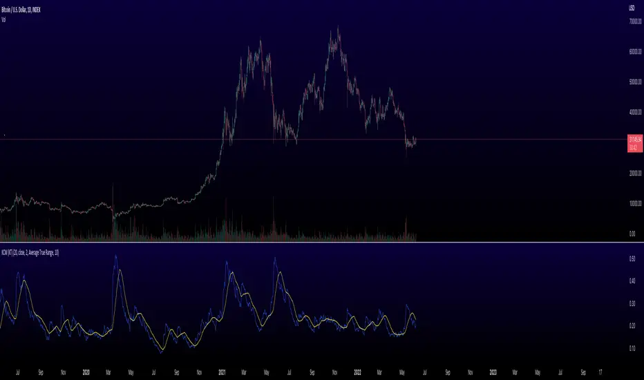
Keltner Channel Width Oscillator (KingThies)Definition
The Keltner Channel Width oscillator is a technical analysis indicator derived originally from the same relationship the Bollinger Band Width indicator takes on Bollinger Bands.
Similar to the Bollinger Bands, Kelts measure volatility in relation to price, and factor in various range calculations to create three bands around the price of a given stock or digital asset. The Middle Line is typically a 20 Day Exponential Moving Average while the upper and lower bands highlight price at different range variations around its basis. Keltner Channel Width serve as a way to quantitatively measure the width between the Upper and Lower Bands and identify opportunities for entires and exits, based on the relative range price is experiencing that day.
Calculation
Kelt Channel Width = (Upper Band - Lower Band) / Middle Band
More on Keltner Channels
Keltner channel was first described by a Chicago grain trader called Chester W. Keltner in his 1960 book How to Make Money in Commodities. Though Keltner claimed no ownership of the original idea and simply called it the ten-day moving average trading rule, his name was applied by those who heard of this concept through his books.
Similarly to the Bollinger Bands, Keltner channel is a technical analysis tool based on three parallel lines. In fact, the Keltner indicator consists of a central moving average in addition to channel lines spread above and below it. The central line represents a 10-day simple moving average of what Chester W. Keltner called typical price. The typical price is defined as the average of the high, low and close. The distance between the central line and the upper, or lower line, is equivalent to the simple moving average of the preceding 10 days' trading ranges.
One way to interpret the Keltner Channel would be to consider the price breakouts outside of the channel. A trader would track price movement and consider any close above the upper line as a strong buy signal. Equivalently, any close below the lower line would be considered a strong sell signal. The trader would follow the trend emphasized by the indicator while complementing his analysis with the use of other indicators as well. However, the breakout method only works well when the market moves from a range-bound setting to an established trend. In a trend-less configuration, the Keltner Channel is better used as an overbought/oversold indicator. Thus, as the price breaks out below the lower band, a trader waits for the next close inside the Keltner Channel and considers this price behavior as an oversold situation indicating a potential buy signal. Similarly, as the price breaks out above the upper band, the trader waits for the next close inside the Keltner Channel and considers this price action as an overbought situation indicating a potential sell signal. By waiting for the price to close within the Channel, the trader avoids getting caught in a real upside or downside breakout.
חפש סקריפטים עבור "bollingerband"
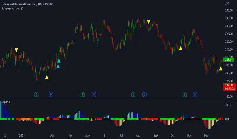
LNL Squeeze ArrowsIf you struggle with the entries, low % win rate or trading the squeeze setup overall, this indicator is for you!
If you look closely at your losing trades, chances are the losers have one thing in common = inverse momentum. I created this tool after I found out that Stacked EMAs and picture perfect trend is not the only thing you need for a squeeze setup. Squeeze arrows pinpoint the exact moment where the squeeze momentum change happens (momentum change is absolutely crucial for the squeeze setup). These arrows will help you stay out of "everything was aligned but still failed" type of setups.
Squeeze Arrows:
1. Momentum Arrows (cyan blue/red) - Showing the best possible moment for an entry during the squeeze (after you see one, you can expect the squeeze to fire soon).
2. Slingshot Arrows (yellow) - Even though you can trade off of them, these arrows work mostly as a confirmation & caution tool. If an inverse slingshot arrow is plotted during a squeeze that means caution = you should wait because momentum is not on your side thus there there is a quite high probability that the squeeze can fire the other direction.
Squeeze Dots Trigger:
Represents the number of red dots (squeeze) after which the arrows should plot. Default = 5 (only after 5 red dots, arrows will appear), some traders like to set it on 3 or even 1.
Tips & Tricks:
1.Breakout or Bailout Mentality
- The big advantage of the arrows is the fact that they either work straight away or they don't. This is where you can apply the breakout or bailout mentality and really focus exclusively on the breakout part of the whole squeeze move. You can minimize the risk by putting mental stops just a few points below the last low of the candle where the arrows appeared. That way you can be stopped out even during the squeeze = won't hurt as much as when the squeeze fire the opposite direction. Reward may be the same but the risk is lower.
2. Yellow Flags
- Use the slingshot arrows as a caution tool. Even if all your squeeze criteria are met. Yellow inverse arrow = caution (wait for the true momentum change). Once the slingshot arrow appears in the conext of the trend, you are good to go.
3. Last Arrow Rule
- Sometimes you will see a lot of arrows during the longer squeezes. This is where the last arrow rule come in handy. The last arrow you see on chart can be canceled anytime by a new one. The last arrow is the valid one!
Hope you can squeeze from these squeeze arrows as much as there is to squeeze so you can finally trade the squeeze with ease.
Hope it helps.
Waddah Attar Explosion V3 [NHK] -Bollinger - MACDWaddah Attar Explosion Version3 indicator to work in Forex and Crypto, This indicator oscillates above and below zero and the Bollinger band is plotted over the MACD Histogram to take quick decisions, Colors are changed for enhanced look. dead zone is plotted in a background area and option is provided to hide dead zone. One can easily detect sideways market movement using Bollinger band and volume. when volume is in between Bollinger band no trades are to be taken as volume is low and market moving in sideways
credits to: @shayankm and @LazyBear
Read the main description below...
- - - - - - - - - - - - - - - - - - - - - - - - - - - - - - - - - - - - - - -
This is a port of a famous MT4 indicator. This indicator uses MACD /BB to track trend direction and strength. Author suggests using this indicator on 30mins.
Explanation from the indicator developer:
"Various components of the indicator are:
Dead Zone Line: Works as a filter for weak signals. Do not trade when the up or down histogram is in between Dead Zone.
Histograms:
- Pink histogram shows the current down trend.
- Blue histogram shows the current up trend.
- Sienna line / Bollinger Band shows the explosion in price up or down.
Signal for ENTER_BUY: All the following conditions must be met.
- Blue histogram is raising.
- Blue histogram above Explosion line.
- Explosion line raising.
- Both Blue histogram and Explosion line above DeadZone line.
Signal for EXIT_BUY: Exit when Blue histogram crosses below Explosion line / Bollinger Band.
Signal for ENTER_SELL: All the following conditions must be met.
- Pink histogram is raising.
- Pink histogram above Explosion line.
- Explosion line raising.
- Both Pink histogram and Explosion line above DeadZone line.
Signal for EXIT_SELL: Exit when Pink histogram crosses below Explosion line.
All of the parameters are configurable via options page. You may have to tune it for your instrument.

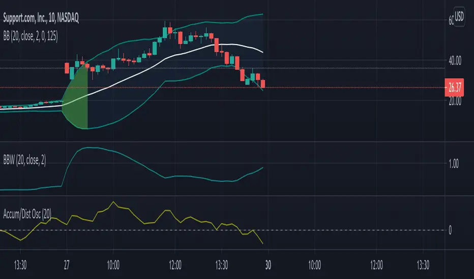
Bollinger Bands w/ Squeeze AlertBollinger's "simple" explanation for a Squeeze is the lowest volatility in the last 6 months. This indicator uses a default look-back period of 125 bars to determine the lowest BandWidth. When current BandWidth drops below the lowest BandWidth of the look-back period, the background of the bands turns red. Default look-back of 125 bars is ~6 months on daily charts.
The source, length, and standard deviation for the Bollinger Bands can all be adjusted. The look-back period for the Squeeze indicator can be adjusted as well.
The image shows my Bollinger Bands w/ Squeeze Alert indicator next to someone else's Bollinger Bandwidth w/ Squeeze Alert indicator to demonstrate how it appears on the chart.
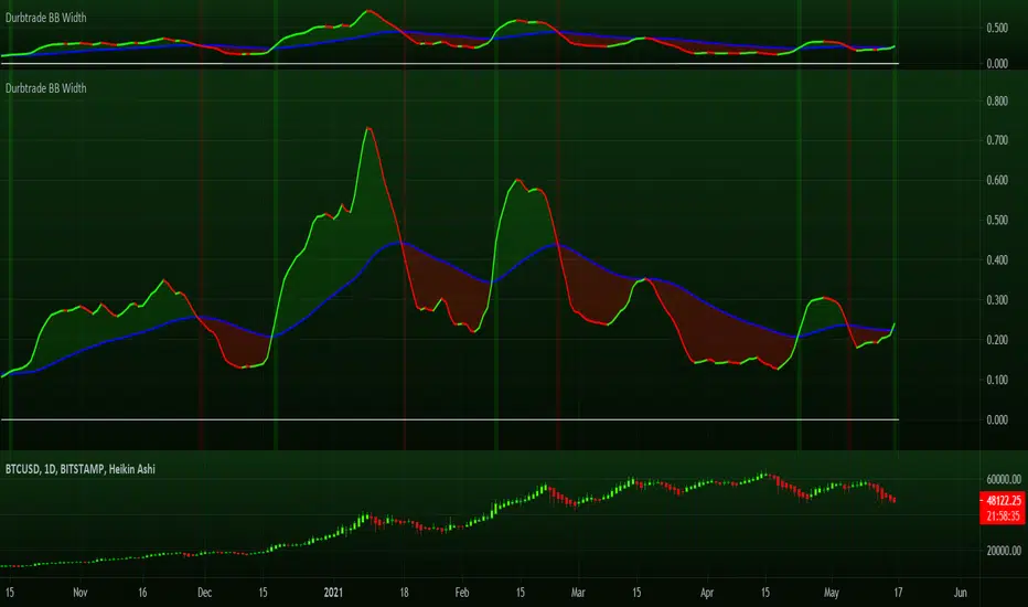
Durbtrade Bollinger Bands WidthFirst published script. Actually, this is my 1st script ever! I know its not flashy or anything, but I finally decided to try learning some pine... and to try and get rid of the dang 0 on my profile, haha. So here are the results after many hours.
I like using the BB Width indicator, and I wanted it to change color based on whether is was rising or falling. I also have it to automatically plot a horizontal line at 0 so I don't have to draw a line every time I apply the indicator to a new chart. And I changed the default precision to 3.
I noticed that there aren't that many BB Width scripts. and I don't think there is anything like this out there that I know of, so I hope someone else besides me will find it useful.
Please feel free to comment.
TradeChartist Risk Meter™𝗧𝗿𝗮𝗱𝗲𝗖𝗵𝗮𝗿𝘁𝗶𝘀𝘁 𝗥𝗶𝘀𝗸 𝗠𝗲𝘁𝗲𝗿 is a very useful and a well designed indicator, that packs a range of Risk utility tools including Trend Based Stochastic Oscillator, Bollinger Bands %B , Volatility Risk Oscillator, RSI Oscillator and RSI Risk Oscillator, along with further visual risk assessment tools like Divergence Spotter, Trend based Strength detector among other useful extras.
===================================================================================================================
™𝗧𝗿𝗮𝗱𝗲𝗖𝗵𝗮𝗿𝘁𝗶𝘀𝘁 𝗥𝗶𝘀𝗸 𝗠𝗲𝘁𝗲𝗿 𝗨𝘀𝗲𝗿 𝗠𝗮𝗻𝘂𝗮𝗹
The user can choose from one of the following four option from the 𝗥𝗶𝘀𝗸 𝗠𝗲𝘁𝗲𝗿 𝗧𝘆𝗽𝗲 dropdown from the settings.
1. Trend Based Stochastic
2. Bollinger Bands %B
3. Volatility Risk Oscillator
4. RSI + RSI Risk Oscillator
The source price for the Risk Meter can be chosen from Sᴏᴜʀᴄᴇ dropdown. Both Trend Based Stochastic and Volatility Risk Oscillator use High/Low prices as default. Enable Usᴇ Sᴏᴜʀᴄᴇ Pʀɪᴄᴇ under respective section to use a different source price.
Users can choose to plot Risk Meter background fill by enabling or disabling Rɪsᴋ Mᴇᴛᴇʀ Bᴀᴄᴋɢʀᴏᴜɴᴅ . The background fill is based on the trend intensity and uses 2 different colour schemes based on user preference. When the Dᴇᴄɪᴅᴇʀ Tʜʀᴇsʜᴏʟᴅ is used, it uses the background fill to mask the zone. If background fill is disabled, orange colour is used to mask the zone.
All of the Risk Meter plots can be plotted as Line , Histogram or Area plots and each of the sections include the Pʟᴏᴛ Sᴛʏʟᴇ option, so the user can choose a specific type of plot style for each of the Risk Meter Oscillators, based on user preference.
===================================================================================================================
═══ 𝟭. 𝗧𝗿𝗲𝗻𝗱 𝗕𝗮𝘀𝗲𝗱 𝗦𝘁𝗼𝗰𝗵𝗮𝘀𝘁𝗶𝗰 ═══
Trend Based Stochastic Oscillator is a modified version of the classic Stochastic Oscillator with the difference being the limits and also the plot itself to an extent.
--> Trend based Stochastic is a single plot oscillates between -100 to +100 and occasionally breaches these limits and can signal extremely overbought or oversold conditions unlike classic Stochastic indicator, which has two plots and strictly oscillates between 0-100.
--> Trend based Stochastic is extremely sensitive to price action, making it possible to detect every single divergence, both regular and hidden, even with the default smoothing factor of 5
--> Risk Meter employs Dᴇᴄɪᴅᴇʀ Tʜʀᴇsʜᴏʟᴅ to let user choose the threshold limit and only from this point onwards, Risk Meter detects the divergences. This helps filter a lot of noise in addition to Price and Oscillator Pivot detection under 𝗗𝗶𝘃𝗲𝗿𝗴𝗲𝗻𝗰𝗲𝘀 section.
The user has to choose the length for the Trend based Stochastic plot by entering number of bars in Lᴏᴏᴋʙᴀᴄᴋ Lᴇɴɢᴛʜ input box (Default value is 55). The user can also change the smoothing factor from default value of 5 by entering the value in Sᴍᴏᴏᴛʜɪɴɢ input box. Smoothing is particularly useful to detect the strength, based on the trend if 𝐂𝐨𝐥𝐨𝐫 𝐙𝐨𝐧𝐞𝐬 𝐛𝐚𝐬𝐞𝐝 𝐨𝐧 𝐒𝐭𝐫𝐞𝐧𝐠𝐭𝐡 is enabled and the required trend length is entered in Tʀᴇɴᴅ Sᴛʀᴇɴɢᴛʜ Dᴇᴛᴇᴄᴛɪᴏɴ Lᴇɴɢᴛʜ . This feature splits the Risk Meter Plot into Bull and Bear zones based on the trend strength. HIgher Smoothing with default trend strength detection of 5 (upto 10) works well for sensitive price hugging scalps/swings. For longer trends, higher detection lengths can be used.
===================================================================================================================
════ 𝟮. 𝗕𝗼𝗹𝗹𝗶𝗻𝗴𝗲𝗿 𝗕𝗮𝗻𝗱𝘀 %𝗕 ═════
Bollinger Bands %B in Risk Meter oscillates between -100 to +100 rather than 0 - 1 in the classic version, with oversold/overbought levels breaching the limits and the plot is exactly the same otherwise.
Risk Meter employs Dᴇᴄɪᴅᴇʀ Tʜʀᴇsʜᴏʟᴅ for Bollinger Bands %B to let the user choose the threshold limit and only from this point onwards, Risk Meter detects the divergences. This helps filter a lot of noise in addition to Price and Oscillator Pivot detection under 𝗗𝗶𝘃𝗲𝗿𝗴𝗲𝗻𝗰𝗲𝘀 section.
The user has to choose the Simple Moving Average (SMA) length for the plot by entering number of bars in BB SMA Lᴇɴɢᴛʜ input box (Default value is 20). There is no need for Standard Deviation as the fundamental plot is exactly the same, given that the plot oscillates between -100 to +100. The user can also change the smoothing factor from default value of 5 by entering the value in Sᴍᴏᴏᴛʜɪɴɢ input box. Smoothing is particularly useful to detect the strength, based on the trend if 𝐂𝐨𝐥𝐨𝐫 𝐙𝐨𝐧𝐞𝐬 𝐛𝐚𝐬𝐞𝐝 𝐨𝐧 𝐒𝐭𝐫𝐞𝐧𝐠𝐭𝐡 is enabled and the required trend length is entered in Tʀᴇɴᴅ Sᴛʀᴇɴɢᴛʜ Dᴇᴛᴇᴄᴛɪᴏɴ Lᴇɴɢᴛʜ . This feature splits the Risk Meter Plot into Bull and Bear zones based on the trend strength. HIgher Smoothing with default trend strength detection of 5 (upto 10) works well for sensitive price hugging scalps/swings. For longer trends, higher detection lengths can be used.
===================================================================================================================
══════ 𝟯. 𝗩𝗼𝗹𝗮𝘁𝗶𝗹𝗶𝘁𝘆 𝗥𝗶𝘀𝗸 ═══════
Volatility Risk Oscillator is an original ™TradeChartist model designed to visually see the Volatility risk for the security on any time frame.
To plot Volatility Risk for the security, the user has to enter the number of bars to detect volatility risk in Lᴏᴏᴋʙᴀᴄᴋ Lᴇɴɢᴛʜ input box (Default Value is 55). The user can also change the smoothing factor from default value of 5 by entering the value in Sᴍᴏᴏᴛʜɪɴɢ input box. Smoothing is particularly useful to detect the strength based on trend if 𝐂𝐨𝐥𝐨𝐫 𝐙𝐨𝐧𝐞𝐬 𝐛𝐚𝐬𝐞𝐝 𝐨𝐧 𝐒𝐭𝐫𝐞𝐧𝐠𝐭𝐡 is enabled and required trend length is entered in Tʀᴇɴᴅ Sᴛʀᴇɴɢᴛʜ Dᴇᴛᴇᴄᴛɪᴏɴ Lᴇɴɢᴛʜ . This feature splits the Risk Meter Plot into Bull and Bear zones based on the trend strength. HIgher Smoothing with default trend strength detection of 5 (upto 10) works well for sensitive price hugging scalps/swings. For longer trends, higher detection lengths can be used.
Even though Divergences work on Volatility Risk Oscillator, it is not employed as it produces far too many and there is no set Threshold limit that can be set to filter the divergences.
===================================================================================================================
══════ 𝟰. 𝗥𝗦𝗜 𝗢𝘀𝗰𝗶𝗹𝗹𝗮𝘁𝗼𝗿 ═══════
There are two different types of RSI Oscillators in this section that can be plotted.
RSI Oscillator - Classic RSI modified to fit -100 to +100 scale rather than 0 - 100 scale. Risk Meter employs Dᴇᴄɪᴅᴇʀ Tʜʀᴇsʜᴏʟᴅ for RSI Oscillator also, to let the user choose the threshold limit and only from this point onwards, Risk Meter detects the divergences. This helps filter a lot of noise in addition to Price and Oscillator Pivot detection under 𝗗𝗶𝘃𝗲𝗿𝗴𝗲𝗻𝗰𝗲𝘀 section.
RSI Risk Oscillator - This oscillator plots the potential RSI risk based on RSI length (which can be changed in RSI Lᴇɴɢᴛʜ input box and main source price ( Sᴏᴜʀᴄᴇ ). The user can also change the smoothing factor from default value of 5 by entering the value in Sᴍᴏᴏᴛʜɪɴɢ input box. Smoothing is particularly useful to detect the strength, based on the trend if 𝐂𝐨𝐥𝐨𝐫 𝐙𝐨𝐧𝐞𝐬 𝐛𝐚𝐬𝐞𝐝 𝐨𝐧 𝐒𝐭𝐫𝐞𝐧𝐠𝐭𝐡 is enabled and the required trend length is entered in Tʀᴇɴᴅ Sᴛʀᴇɴɢᴛʜ Dᴇᴛᴇᴄᴛɪᴏɴ Lᴇɴɢᴛʜ . This feature splits the Risk Meter Plot into Bull and Bear zones based on the trend strength. Higher Smoothing with default trend strength detection of 5 (upto 10) works well for sensitive price hugging scalps/swings. For longer trends, higher detection lengths can be used.
To plot RSI Risk Oscillator, 𝐒𝐡𝐨𝐰 𝐑𝐒𝐈 𝐑𝐢𝐬𝐤 𝐎𝐬𝐜𝐢𝐥𝐥𝐚𝐭𝐨𝐫 must be enabled. Disabling this option plots normal RSI Oscillator.
The 4hr chart of BTC-USDT below shows use of RSI Risk Oscillator (Top) with RSI Oscillator (bottom).
===================================================================================================================
╔═══════ 𝗗𝗶𝘃𝗲𝗿𝗴𝗲𝗻𝗰𝗲𝘀 ═══════╗
Risk Meter detects both Regular and Hidden Bullish and Bearish Divergences at every occurence. This can be filtered by the use of Dᴇᴄɪᴅᴇʀ Tʜʀᴇsʜᴏʟᴅ in above sections. To plot divergences, enable
𝗗𝗶𝘃𝗲𝗿𝗴𝗲𝗻𝗰𝗲𝘀, Sʜᴏᴡ Rᴇɢᴜʟᴀʀ Dɪᴠᴇʀɢᴇɴᴄᴇs and Sʜᴏᴡ Hɪᴅᴅᴇɴ Dɪᴠᴇʀɢᴇɴᴄᴇs . All divergences are enabled as default.
Users can further filter Divergences by entering the number of bars to the right in Rɪɢʜᴛ ʙᴀʀs ғᴏʀ Pɪᴠᴏᴛ Cᴏɴғɪʀᴍᴀᴛɪᴏɴ input box to confirm the Price Pivot (for Regular divergences) and Oscillator Pivot (for Hidden Divergences).
The example chart of 4hr BTC-USDT chart shows the Divergences filtered by use of RSI Threshold. It is important to note that the trend intensity colour on the plot and bars (if bar colour option is enabled) will help detect if the Divergence would hold.
===================================================================================================================
╔═══════ 𝗨𝘀𝗲𝗳𝘂𝗹 𝗘𝘅𝘁𝗿𝗮𝘀 ═══════╗
Risk Meter offer two vibrant Colour Themes, namely Chilli and Flame , which can be opted from Rɪsᴋ Mᴇᴛᴇʀ Tʜᴇᴍᴇ dropdown. These themes also offer the option to plot the trend intensity on the price bars as bar colours by enabling Rɪsᴋ Mᴇᴛᴇʀ Cᴏʟᴏᴜʀ Bᴀʀs . Bar colors can also be inverted using Iɴᴠᴇʀᴛ Bᴀʀ Cᴏʟᴏᴜʀ option.
Users can also choose to use the Simple theme and choose preferred colours from Sɪᴍᴘʟᴇ Tʜᴇᴍᴇ ʙᴜʟʟ Cᴏʟᴏᴜʀ and Sɪᴍᴘʟᴇ Tʜᴇᴍᴇ ʙᴇᴀʀ Cᴏʟᴏᴜʀ colour input.
Note: The indicator does not repaint and can be confidently used for alerts and trade entries without worrying about plots disappearing after bar close.
===================================================================================================================
Example Charts
1. 89 period Trend Based Stochastic Oscillator as Histogram plot on LINK-USDT 1hr chart with Chilli Theme.
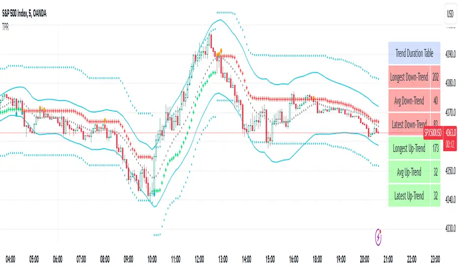
2. 89 period Volatility Risk Oscillator as Histogram plot on SPX 1hr chart with Chilli Theme.
3. 14 period RSI Risk Oscillator as Area plot on AAPL Daily Chart with Flame Theme.
4. 100 period Volatility Risk Oscillator using Trend Strength plotted as Zones on 1hr EUR-USD chart with Chilli Theme.
===================================================================================================================
Best Practice: Test with different settings first using Paper Trades before trading with real money
===================================================================================================================
This is not a free to use indicator. Get in touch with me (PM me directly if you would like trial access to test the indicator)
Premium Scripts - Trial access and Information
Trial access offered on all Premium scripts.
PM me directly to request trial access to the scripts or for more information.
===================================================================================================================

[blackcat] L2 Center Band BollingerLevel: 2
Background
Bollinger bands are a type of price envelope developed by John Bollinger , where price envelopes define upper and lower price ranges. Bollinger Bands are envelopes that are represented with a standard deviation above and below a simple moving average of price. Because the spacing of the bands is based on the standard deviation, they adjust for fluctuations in the volatility of the underlying price.
Function
L2 Center Band Bollinger takes advantage of Bollinger band to detect sideways and trends. At the same time, I made an improvement and the center Bollinger line as a fast-slow-line color band. The algorithm of the color center band is composed of price and volume information, which produces gold cross and dead cross for short term long and short entries.
Key Signal
aa10 --> bollinger middle fast line
aa12 --> bollinger middle slow line
up --> upper envelope
dn --> lower envelope
Pros and Cons
Pros:
1. it can easy see the sections of trends or sideways by width of Bollinger band
2. long and short entries are disclosed
Cons:
1. Some noise is still incorporated in trends
2. due to this is un-optimized version, time frame and trading pairs need to be selected
3. Bollinger re-entry signal is not disclosed yet
Remarks
The long and short signal is compatible to @nilux strategy backtest framework for sandardized backtest scheme: Backtest
Readme
In real life, I am a prolific inventor. I have successfully applied for more than 60 international and regional patents in the past 12 years. But in the past two years or so, I have tried to transfer my creativity to the development of trading strategies. Tradingview is the ideal platform for me. I am selecting and contributing some of the hundreds of scripts to publish in Tradingview community. Welcome everyone to interact with me to discuss these interesting pine scripts.
The scripts posted are categorized into 5 levels according to my efforts or manhours put into these works.
Level 1 : interesting script snippets or distinctive improvement from classic indicators or strategy. Level 1 scripts can usually appear in more complex indicators as a function module or element.
Level 2 : composite indicator/strategy. By selecting or combining several independent or dependent functions or sub indicators in proper way, the composite script exhibits a resonance phenomenon which can filter out noise or fake trading signal to enhance trading confidence level.
Level 3 : comprehensive indicator/strategy. They are simple trading systems based on my strategies. They are commonly containing several or all of entry signal, close signal, stop loss, take profit, re-entry, risk management, and position sizing techniques. Even some interesting fundamental and mass psychological aspects are incorporated.
Level 4 : script snippets or functions that do not disclose source code. Interesting element that can reveal market laws and work as raw material for indicators and strategies. If you find Level 1~2 scripts are helpful, Level 4 is a private version that took me far more efforts to develop.
Level 5 : indicator/strategy that do not disclose source code. private version of Level 3 script with my accumulated script processing skills or a large number of custom functions. I had a private function library built in past two years. Level 5 scripts use many of them to achieve private trading strategy.

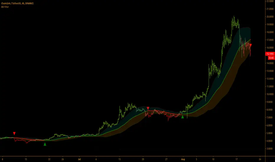
Bollinger Bands Filter
Bollinger Bands is a classic indicator that uses a simple moving average of 20 periods, along with plots of upper and lower bands that are 2 standard deviations away from the basis line. These bands help visualize price volatility and trend based on where the price is, in relation to the bands.
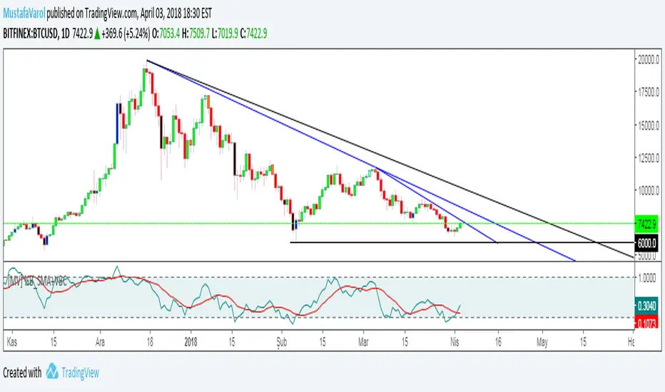
Bollinger Bands filter plots a long signal when price closes above the upper band and plots a short signal when price closes below the lower band. It doesn't take into account any other parameters such as Volume/RSI/ Fundamentals etc, so user must use discretion based on confirmations from another indicator or based on fundamentals.
The filter works great when the price closes above/below upper/lower bands with continuation on next bar. It is definitely useful to have this filter along with other indicators to get early glimpse of breach/fail of bands on candle close during BB squeeze or based on volatility.
This can be used on Heikin Ashi candles for spotting trends, but HA candles are not recommended for trade entries as they don't reflect true price of the asset.
This filter's default is 55 SMA and 1 standard deviation, but these can be changed from settings.
It is definitely worth reading the 22 rules of Bollinger Bands written by John Bollinger.
==================================================================
Note:
1. Alerts can be created for long and short signals using "Once per bar close".
2. The indicator doesn't repaint.
==================================================================
Colored Directional Movement and Bollinger Band's Cloud by DGTThis study combines Bollinger Bands, one of the most popular technical analysis indicators on the market, and Directional Movement (DMI), which is another quite valuable technical analysis indicator.
Bollinger Bands used in conjunction with Directional Movement (DMI) may help getting a better understanding of the ever changing landscape of the market and perform more advanced technical analysis
Here are details of the concept applied
1- Plots Bollinger Band’s (BB) Cloud colored based on Bollinger Band Width (BBW) Indicator’s value
Definition
Bollinger Bands (created by John Bollinger ) are a way to measure volatility . As volatility increases, the wider the bands become and similarly as volatility decreases, the gap between bands narrows
Bollinger Bands, in widely used approach, consist of a band of three lines. Likewise common usage In this study a band of five lines is implemented
The line in the middle is a Simple Moving Average (SMA) set to a period of 20 bars (the most popular usage). The SMA then serves as a base for the Upper and Lower Bands. The Upper and Lower Bands are used as a way to measure volatility by observing the relationship between the Bands and price. the Upper and Lower Bands in this study are set to two and three standard deviations (widely used form is only two standard deviations) away from the SMA (The Middle Line), hence there are two Upper Bands and two Lower Bands. The background between two Upper Bands is filled with a green color and the background between two Lower Bands is filled with a red color. In this we have obtained Bollinger Band’s (BB) Clouds (Upper Cloud and Lower Cloud)
Additionally the intensity of the color of the background is calculated with Bollinger Bands Width ( BBW ), which is a technical analysis indicator derived from the standard Bollinger Bands indicator. Bollinger Bands Width, quantitatively measures the width between the Upper and Lower Bands. In this study the intensity of the color of the background is increased if BBW value is greater than %25
What to look for
Price Actions : Prices are almost always within the bands especially at this study the bands of three standard deviations away from the SMA. Price touching or breaking the BB Clouds could be considered as buying or selling opportunity. However this is not always the case, there are exceptions such as Walking the Bands. “Walking the Bands” can occur in either a strong uptrend or a strong downtrend. During a strong trend, there may be repeated instances of price touching or breaking through the BB Clouds. Each time that this occurs, it is not a signal, it is a result of the overall strength of the move. In this study in order to get a better understanding of the trend and add ability to perform some advanced technical analysis Directional Movement Indicator (DMI) is added to be used in conjunction with Bollinger Bands.
Cycling Between Expansion and Contraction : One of the most well-known theories in regards to Bollinger Bands is that volatility typically fluctuates between periods of expansion (Bands Widening : surge in volatility and price breaks through the BB Cloud) and contraction (Bands Narrowing : low volatility and price is moving relatively sideways). Using Bollinger Bands in conjunction with Bollinger Bands Width may help identifying beginning of a new directional trend which can result in some nice buying or selling signals. Of course the trader should always use caution
2- Plots Colored Directional Movement Line
Definition
Directional Movement (DMI) (created by J. Welles Wilder ) is actually a collection of three separate indicators combined into one. Directional Movement consists of the Average Directional Index (ADX) , Plus Directional Indicator (+D I) and Minus Directional Indicator (-D I) . ADX's purposes is to define whether or not there is a trend present. It does not take direction into account at all. The other two indicators (+DI and -DI) are used to compliment the ADX. They serve the purpose of determining trend direction. By combining all three, a technical analyst has a way of determining and measuring a trend's strength as well as its direction.
This study combines all three lines in a single colored shapes series plotted on the top of the price chart indicating the trend strength with different colors and its direction with triangle up and down shapes.
What to look for
Trend Strength : Analyzing trend strength is the most basic use for the DMI. Wilder believed that a DMI reading above 25 indicated a strong trend, while a reading below 20 indicated a weak or non-existent trend
Crosses : DI Crossovers are the significant trading signal generated by the DMI
With this study
A Strong Trend is assumed when ADX >= 25
Bullish Trend is defined as (+D I > -DI ) and (ADX >= 25), which is plotted as green triangle up shape on top of the price chart
Bearish Trend is defined as (+D I < -DI ) and (ADX >= 25), which is plotted as red triangle down shape on top of the price chart
Week Trend is assumed when 17< ADX < 25, which is plotted as black triangles up or down shape, depending on +DI-DI values, on top of the price chart
Non-Existent Trend is assumed when ADX < 17, which is plotted as yellow triangles up or down shape, depending on +DI-DI values, on top of the price chart
Additionally intensity of the colors used in all cases above are defined by comparing ADX’s current value with its previous value
Summary of the Study:
Even more simplified and visually enhanced DMI drawing comparing to its classical usage (may require a bit practice to get used to it)
As said previously, to get a better understanding of the trend and add ability to perform some advanced technical analysis Directional Movement Indicator (DMI) is used in conjunction with Bollinger Bands.
PS: Analysis and tests are performed with high volatile Cryptocurrency Market
Source of References : definitions provided herein are gathered from TradingView’s knowledgebase/library
Disclaimer: The script is for informational and educational purposes only. Use of the script does not constitutes professional and/or financial advice. You alone the sole responsibility of evaluating the script output and risks associated with the use of the script. In exchange for using the script, you agree not to hold dgtrd tradingview user liable for any possible claim for damages arising from any decision you make based on use of the script

Turtle IndexThis Indicator is a combination of Super Smoother Filter and Bollinger Bands %B.
This Indicator is used in Trend-Momentum gauging. Use this indicator with Turtle Oscillator.


Tran Truong indicatorChỉ báo tìm điểm vào ra thị trường dựa trên phân kỳ hội tụ
bao gồm ichimoku, bollingerband

[NMC]RSI MTF, StochasticRSI MTF, BB%, WavetrendThis is our second indicator and is very useful if you want to create a strategy based on multiple indicators and time frames. RSI and Stochastic RSI are multi-timeframe and they are based on ChrisMoody's multi-timeframe scripts.
You can choose from RSI, Stochastic RSI, BB% and Wavetrend. In the near future we my add CCI, CMF, TSI or any similar indicator with the possibility to plot from a higher timeframe.
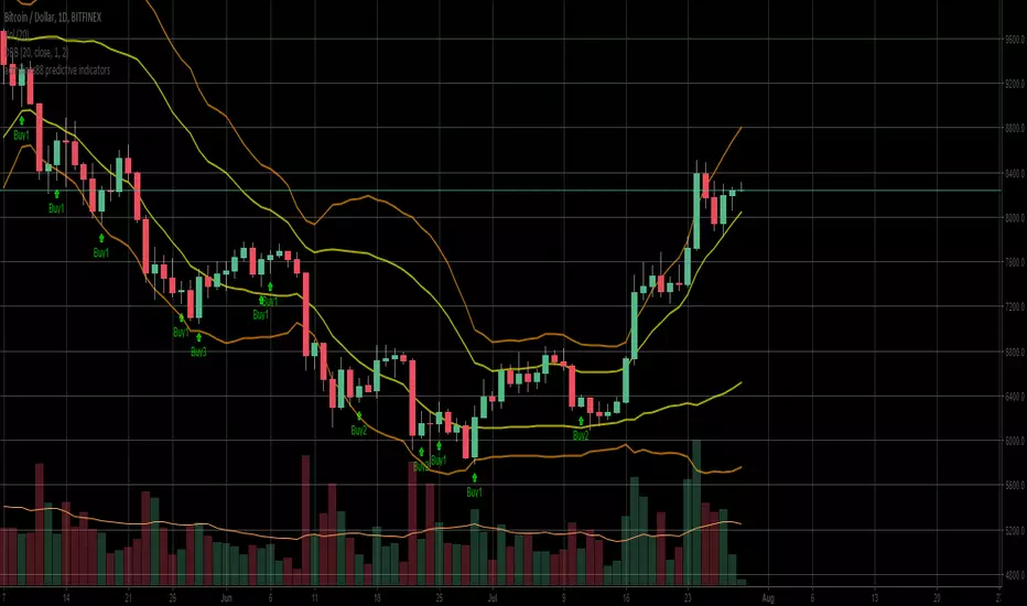
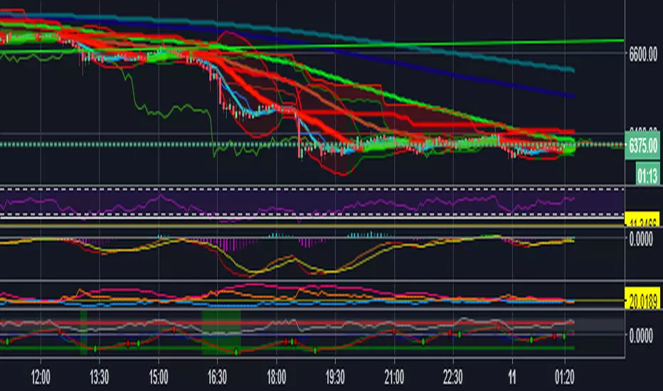
acmillions88 predictive indicatorsUnlike most scripts, this script actually predicts the mini trends. Works great with double bollingerbands.
6xMa_ichimoku_MTF_Boll_SuperTrend V2 update [PlungerMen]hello!
This script very funny :))
This Script version update , I made for a friend named Huu Trung You can add to it This script have 3 ema , 3 wma , bollingerBand super Trend, Ichimokhu, mtf ma In settings there is a section to turn off what you do not like Hope you enjoy this version
6x MA in one Chart
You can change color, hide Ma if you want
Ichimoku Clound
MTF indicator
Boolinger band and Super trend pro
have you like!
3Ema_3Wma_boll_MTF_ichi [PlungerMen]hello !
This Script version I made for a friend named Huu Trung
You can add to it
This script have
3 ema ,
3 wma ,
bollingerBand super Trend,
Ichimokhu,
mtf ma
In settings there is a section to turn off what you do not like
Hope you enjoy this version

[MV] %B with SMA + Volume Based Colored Bars
Entry Signal when %B Crosses with SMA and this is more meaningful if it supports colored bars.
Black Bar when prices go down and volume is bigger than 150% of its average, that indicates us price action is supported by a strong bearish volume
Blue Bar when prices go up and volume bigger than 150% of its average, that indicates us price action is supported by a strong bullish volume
VBC author @KIVANCfr3762
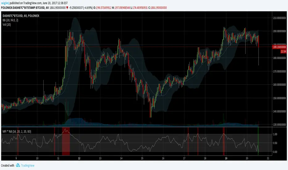
MFI * %B [seiglerj]Oscillator averaging Money Flow Index and Bollinger Bands' %B
Colored bars indicate buy or sell signals
I have no idea if this is the right way to combine these two, but I'm gonna try it and see what happens
Trend Pullback Reversal TPRThe TPR(Trend Pullback Reversal) indicator forms a possible price trend with support and resistance lines. It also comes with a unqiue band and center line as additional features.
TPR works on all timeframes and all symbols and all type of bar chart.
TPR never repaints.
There are 4 Parameters:
Period: umber of bars used for calculations
Factor: Multiplier factor, small number for short trend, large number for long trend
Source: the input series, default is Close
ShowBand: enable to show band and center line
Most trend indicators have similar plot, the difference is where and when they change the direction. Unlike other trend indicators, TPR will focus on main trend and filter out most minor price movements. The green cross-line represents an uptrend, the red cross-line represents a downtrend.
The additional band and center line may look like bollinger band, but the TPR band algorithm is completely different from bollingerband. There is no standard deviation in TPR band calculation.
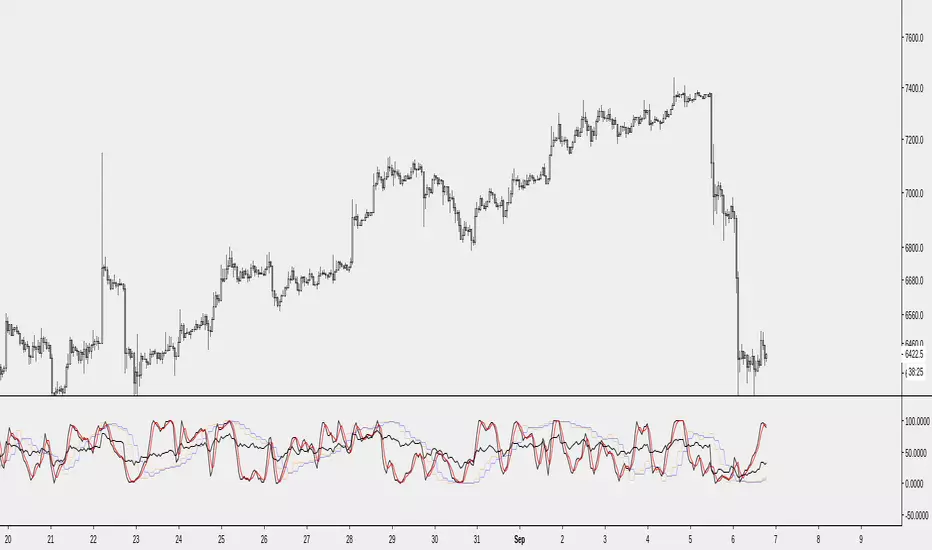
RSI Bands, RSI %B and RSI BandwidthRSI bands provide an intuitive way of visualizing how the price movement causes RSI to move with in its range (0-100). Upper/Lower bands signify overbought and oversold levels respectively (Default: 70/30, you can customize them via options page). These bands closely match what Constance Brown explains in her book "Technical Analysis for the Trading Professional".
I have also coded up 2 scripts to visualize %B and Bandwidth, just as in BollingerBands. As you can see %B is equivalent to the actual RSI. Along with RSI_Bandwidth and %B, the bands convey a lot of information.
Another tip is to render Bollinger Bands along with RSIBands...endless possibilities :)
I have included all 3 scripts in the same chart, as they are all related. Since TradingView doesn't allow sharing more than one script in the same chart, you can only "Add script" RSI Bands.
If you want to use RSI %B and Bandwidth, follow this guide to "Make mine" this chart and get access to the source:
drive.google.com
For the complete list of my indicators, check this post:

Indicators: Traders Dynamic Index, HLCTrends and Trix Ribbon1) Trix Ribbon
===============================================================
This was built on request. Many Stock/FX traders overlay multiple Trix lines to form the ribbon, this indicator makes it easy.
Also, optionally this can plot a BollingerBand on Trix_1.
More info on Trix:
stockcharts.com
2) High/Low/Close Trend Indicator
===============================================================
Simple indicator using EMAs of H/L/C. If blue line is above the red line, the trend is up, else down. Keep an eye on the zero line too.
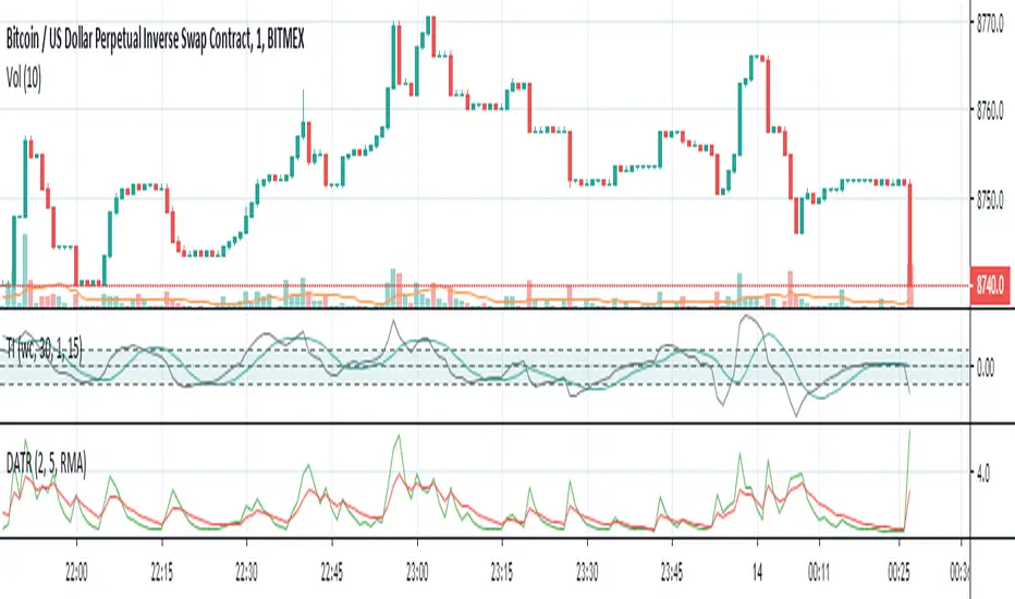
3) Traders Dynamic Index
===============================================================
This hybrid indicator helps to decipher and monitor market conditions related to trend direction, market strength, and market volatility.
TDI has the following components:
* Green line = RSI Price line
* Red line = Trade Signal line
* Blue lines = Volatility Bands
* Orange line = Market Base Line
Trend Direction - Immediate and Overall:
----------------------------------------------------
* Immediate = Green over Red...price action is moving up.
Red over Green...price action is moving down.
* Overall = Orange line trends up and down generally between the lines 32 & 68. Watch for Orange line to bounces off these lines for market reversal. Trade long when price is above the Orange line, and trade short when price is below.
Market Strength & Volatility - Immediate and Overall:
----------------------------------------------------
* Immediate = Green Line - Strong = Steep slope up or down.
Weak = Moderate to Flat slope.
* Overall = Blue Lines - When expanding, market is strong and trending. When constricting, market is weak and in a range. When the Blue lines are extremely tight in a narrow range, expect an economic announcement or other market condition to spike the market.
Entry conditions:
----------------------------------------------------
* Scalping - Long = Green over Red,
Short = Red over Green
* Active - Long = Green over Red & Orange lines
Short = Red over Green & Orange lines
* Moderate - Long = Green over Red, Orange, & 50 lines
Short= Red over Green, Green below Orange & 50 line
Exit conditions:
----------------------------------------------------
If Green crosses either Blue lines, consider exiting when the Green line crosses back over the Blue line.
* Long = Green crosses below Red
* Short = Green crosses above Red
More info on a complete system using TDI:
www.forexmt4.com

VectorCoresAI SMA + Bollinger Fusion v1VectorCoresAI — SMA + Bollinger Fusion (Free)
A clean, modern visual tool combining four key SMAs with an adaptive Bollinger structure.
This script merges two of the most widely used charting concepts into one simple, readable view:
Included
✔ SMA 21
✔ SMA 50
✔ SMA 100
✔ SMA 200
✔ Bollinger Bands with adjustable length + multiplier
✔ Adaptive “Fusion Squeeze” shading to highlight compression phases
✔ Optional visibility toggles for each SMA
✔ Lightweight, non-intrusive overlay
What this indicator is designed for
This tool helps traders quickly understand:
Trend alignment using the 21/50/100/200 SMAs
Volatility conditions around the Bollinger midline
Price compression and expansion
Early awareness of breakout environments
Clean visual structure without clutter
Everything is intentionally simple and transparent.
No predictions, no signals, no trading advice — just clean chart structure.
Why this version is unique
Instead of using standard Bollinger visuals, this Fusion edition uses subtle adaptive shading to show when the bands contract.
This makes compression zones instantly visible without overwhelming the chart.
The SMAs are fixed to widely-used trend levels, giving consistent readings across all markets and timeframes.
Who this is for
Newer traders who want a clear introduction to SMAs + Bollinger Bands
Experienced traders who want a lightweight visual tool
Anyone building structure-based strategies
Users of the VectorCoresAI suite who want a simple companion tool
Notes
This indicator is part of the VectorCoresAI Free Tools collection.
All logic is open-source and educational only.
More tools coming soon.
