HEMA - A Fast And Efficient Estimate Of The Hull Moving AverageIntroduction
The Hull moving average (HMA) developed by Alan Hull is one of the many moving averages that aim to reduce lag while providing effective smoothing. The HMA make use of 3 linearly weighted (WMA) moving averages, with respective periods p/2 , p and √p , this involve three convolutions, which affect computation time, a more efficient version exist under the name of exponential Hull moving average (EHMA), this version make use of exponential moving averages instead of linearly weighted ones, which dramatically decrease the computation time, however the difference with the original version is clearly noticeable.
In this post an efficient and simple estimate is proposed, the estimation process will be fully described and some comparison with the original HMA will be presented.
This post and indicator is dedicated to LucF
Estimation Process
Estimating a moving average is easier when we look at its weights (represented by the impulse response), we basically want to find a similar set of weights via more efficient calculations, the estimation process is therefore based on fully understanding the weighting architecture of the moving average we want to estimate.
The impulse response of an HMA of period 20 is as follows :
We can see that the first weights increases a bit before decaying, the weights then decay, cross under 0 and increase again. More recent closing price values benefits of the highest weights, while the oldest values have negatives ones, negative weighting is what allow to drastically reduce the lag of the HMA. Based on this information we know that our estimate will be a linear combination of two moving averages with unknown coefficients :
a × MA1 + b × MA2
With a > 0 and b < 0 , the lag of MA1 is lower than the lag of MA2 . We first need to capture the general envelope of the weights, which has an overall non-linearly decaying shape, therefore the use of an exponential moving average might seem appropriate.
In orange the impulse response of an exponential moving average of period p/2 , that is 10. We can see that such impulse response is not a bad estimate of the overall shape of the HMA impulse response, based on this information we might perform our linear combination with a simple moving average :
2EMA(p/2) + -1SMA(p)
this gives the following impulse response :
As we can see there is a clear lack of accuracy, but because the impulse response of a simple moving is a constant we can't have the short increasing weights of the HMA, we therefore need a non-constant impulse response for our linear combination, a WMA might be appropriate. Therefore we will use :
2WMA(p/2) + -1EMA(p/2)
Note that the lag a WMA is inferior to the lag of an EMA of same period, this is why the period of the WMA is p/2 . We obtain :
The shape has improved, but the fit is poor, which mean we should change our coefficients, more precisely increasing the coefficient of the WMA (thus decreasing the one of the EMA). We will try :
3WMA(p/2) + -2EMA(p/2)
We then obtain :
This estimate seems to have a decent fit, and this linear combination is therefore used.
Comparison
HMA in blue and the estimate in fuchsia with both period 50, the difference can be noted, however the estimate is relatively accurate.
In the image above the period has been set to 200.
Conclusion
In this post an efficient estimate of the HMA has been proposed, we have seen that the HMA can be estimated via the linear combinations of a WMA and an EMA of each period p/2 , this isn't important for the EMA who is based on recursion but is however a big deal for the WMA who use recursion, and therefore p indicate the number of data points to be used in the convolution, knowing that we use only convolution and that this convolution use twice less data points then one of the WMA used in the HMA is a pretty great thing.
Subtle tweaking of the coefficients/moving averages length's might help have an even more accurate estimate, the fact that the WMA make use of a period of √p is certainly the most disturbing aspect when it comes to estimating the HMA. I also described more in depth the process of estimating a moving average.
I hope you learned something in this post, it took me quite a lot of time to prepare, maybe 2 hours, some pinescripters pass an enormous amount of time providing content and helping the community, one of them being LucF, without him i don't think you'll be seeing this indicator as well as many ones i previously posted, I encourage you to thank him and check his work for Pinecoders as well as following him.
Thanks for reading !
חפש סקריפטים עבור "one一季度财报"

PivotBoss TriggersI have collected the four PivotBoss indicators into one big indicator. Eventually I will delete the individual ones, since you can just turn off the ones you don't need in the style controller. Cheers.
Wick Reversal
When the market has been trending lower then suddenly forms a reversal wick candlestick , the likelihood of
a reversal increases since buyers have finally begun to overwhelm the sellers. Selling pressure rules the decline,
but responsive buyers entered the market due to perceived undervaluation. For the reversal wick to open near the
high of the candle, sell off sharply intra-bar, and then rally back toward the open of the candle is bullish , as it
signifies that the bears no longer have control since they were not able to extend the decline of the candle, or the
trend. Instead, the bulls were able to rally price from the lows of the candle and close the bar near the top of its
range, which is bullish - at least for one bar, which hadn't been the case during the bearish trend.
Essentially, when a reversal wick forms at the extreme of a trend, the market is telling you that the trend
either has stalled or is on the verge of a reversal. Remember, the market auctions higher in search of sellers, and
lower in search of buyers. When the market over-extends itself in search of market participants, it will find itself
out of value, which means responsive market participants will look to enter the market to push price back toward
an area of perceived value. This will help price find a value area for two-sided trade to take place. When the
market finds itself too far out of value, responsive market participants will sometimes enter the market with
force, which aggressively pushes price in the opposite direction, essentially forming reversal wick candlesticks .
This pattern is perhaps the most telling and common reversal setup, but requires steadfast confirmation in order
to capitalize on its power. Understanding the psychology behind these formations and learning to identify them
quickly will allow you to enter positions well ahead of the crowd, especially if you've spotted these patterns at
potentially overvalued or undervalued areas.
Fade (Extreme) Reversal
The extreme reversal setup is a clever pattern that capitalizes on the ongoing psychological patterns of
investors, traders, and institutions. Basically, the setup looks for an extreme pattern of selling pressure and then
looks to fade this behavior to capture a bullish move higher (reverse for shorts). In essence, this setup is visually
pointing out oversold and overbought scenarios that forces responsive buyers and sellers to come out of the dark
and put their money to work-price has been over-extended and must be pushed back toward a fair area of value
so two-sided trade can take place.
This setup works because many normal investors, or casual traders, head for the exits once their trade
begins to move sharply against them. When this happens, price becomes extremely overbought or oversold,
creating value for responsive buyers and sellers. Therefore, savvy professionals will see that price is above or
below value and will seize the opportunity. When the scared money is selling, the smart money begins to buy, and
Vice versa.
Look at it this way, when the market sells off sharply in one giant candlestick , traders that were short
during the drop begin to cover their profitable positions by buying. Likewise, the traders that were on the
sidelines during the sell-off now see value in lower prices and begin to buy, thus doubling up on the buying
pressure. This helps to spark a sharp v-bottom reversal that pushes price in the opposite direction back toward
fair value.
Engulfing (Outside) Reversal
The power behind this pattern lies in the psychology behind the traders involved in this setup. If you have
ever participated in a breakout at support or resistance only to have the market reverse sharply against you, then
you are familiar with the market dynamics of this setup. What exactly is going on at these levels? To understand
this concept is to understand the outside reversal pattern. Basically, market participants are testing the waters
above resistance or below support to make sure there is no new business to be done at these levels. When no
initiative buyers or sellers participate in range extension, responsive participants have all the information they
need to reverse price back toward a new area of perceived value.
As you look at a bullish outside reversal pattern, you will notice that the current bar's low is lower than the
prior bar's low. Essentially, the market is testing the waters below recently established lows to see if a downside
follow-through will occur. When no additional selling pressure enters the market, the result is a flood of buying
pressure that causes a springboard effect, thereby shooting price above the prior bar's highs and creating the
beginning of a bullish advance.
If you recall the child on the trampoline for a moment, you'll realize that the child had to force the bounce
mat down before he could spring into the air. Also, remember Jennifer the cake baker? She initially pushed price
to $20 per cake, which sent a flood of orders into her shop. The flood of buying pressure eventually sent the price
of her cakes to $35 apiece. Basically, price had to test the $20 level before it could rise to $35.
Let's analyze the outside reversal setup in a different light for a moment. One of the reasons I like this setup
is because the two-bar pattern reduces into the wick reversal setup, which we covered earlier in the chapter. If
you are not familiar with candlestick reduction, the idea is simple. You are taking the price data over two or more
candlesticks and combining them to create a single candlestick . Therefore, you will be taking the open, high, low,
and close prices of the bars in question to create a single composite candlestick .
Doji Reversal
The doji candlestick is the epitome of indecision. The pattern illustrates a virtual stalemate between buyers
and sellers, which means the existing trend may be on the verge of a reversal. If buyers have been controlling a
bullish advance over a period of time, you will typically see full-bodied candlesticks that personify the bullish
nature of the move. However, if a doji candlestick suddenly appears, the indication is that buyers are suddenly
not as confident in upside price potential as they once were. This is clearly a point of indecision, as buyers are no
longer pushing price to higher valuation, and have allowed sellers to battle them to a draw-at least for this one
candlestick . This leads to profit taking, as buyers begin to sell their profitable long positions, which is heightened
by responsive sellers entering the market due to perceived overvaluation. This "double whammy" of selling
pressure essentially pushes price lower, as responsive sellers take control of the market and push price back
toward fair value.

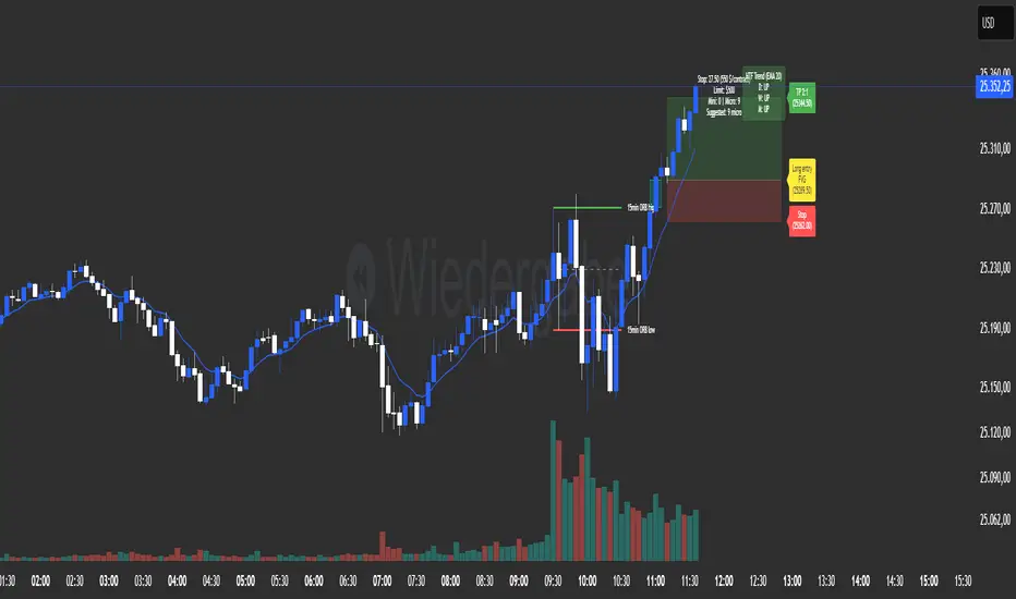
Morning ORB FVG Trigger✅ Overview
Morning ORB FVG Trigger is a complete intraday trading framework built around:
A Morning Opening Range Breakout (ORB)
The first Fair Value Gap (FVG) after that breakout
Strict risk management and position sizing
Optional HTF trend filter (Daily / Weekly / Monthly)
Optional Daily ATR filter to avoid extreme days
The script is designed for futures / indices / FX on intraday charts up to 15 minutes and for traders who want a clean, mechanical entry framework with clear risk.
🧠 Core idea
Define a morning opening range (e.g. 09:30–09:45).
Wait for a clean breakout above/below that range.
After the breakout, wait for the first FVG in breakout direction,
confirmed by the next candle (no immediate full reclaim).
Use a chosen stop logic + R:R factor to build risk/reward boxes.
Calculate position size based on your account risk.
(Optional) Only take trades:
In the direction of the HTF EMA trend (D/W/M).
On days where the morning range is within a band of the Daily ATR.
You can also disable all signals/boxes and use the script just as a visual ORB tool.
⏰ 1. ORB / Morning Range
Inputs (Main section)
Morning Range Session
Time window of the opening range in exchange time
Example: 09:30–09:45 for a 15-minute ORB.
You can type custom ranges (e.g. 09:30–09:35 for a 5-minute ORB).
Risk/Reward (TP factor)
Multiplier for the take-profit distance relative to the stop.
2.0 = TP is 2× the stop distance
1.5 = TP is 1.5× the stop distance
Show ORB range
If enabled, draws:
ORB high/low lines
ORB labels (e.g. 15min ORB high / low)
Optional midline
Extend ORB lines to the right (bars)
How many bars to extend the ORB high/low horizontally beyond the ORB itself.
Trade box width (bars)
Horizontal width (in bars) of:
Red risk box (entry–stop)
Green reward box (entry–TP)
Implementation details
The ORB is always calculated on 1-minute data internally, so it stays precise even on 5m/15m charts.
The script only works on intraday timeframes up to 15 minutes.
📦 2. FVG Block
Group: “FVG”
Threshold %
Minimum size of an FVG in % of price.
0 = every FVG
Higher values = only larger gaps
Auto threshold (from volatility)
If enabled, the minimum FVG size is derived from historical volatility
instead of a fixed percentage.
Allow breakout FVG partly inside ORB
Off (default): the FVG must lie fully outside the ORB.
On: the breakout FVG itself may still overlap the ORB a bit,
as long as it is the first one attached to the breakout move.
Enable FVG entry signals, boxes & alerts
On: full system – FVG detection, entry labels, risk/TP boxes, alerts.
Off: no entries, no risk/TP boxes, no alerts.
You only get the ORB and (optionally) the HTF dashboard, so you can trade your own setups.
Entry mode
Entry mode (Mid / Edge / NextOpen)
Mid – Entry at the midpoint of the FVG.
Edge – Long at the upper FVG edge, short at the lower FVG edge.
NextOpen – No limit order in the gap. Entry is placed at the next bar open after FVG confirmation.
Edge offset (ticks)
Additional offset for Edge entries:
Long:
+ticks = a bit above the FVG (more conservative)
-ticks = deeper into the FVG (more aggressive)
Short:
+ticks = a bit below the FVG
-ticks = deeper into the FVG
FVG detection logic
Uses a LuxAlgo-style 3-candle FVG pattern (gap between candle 1 and 3).
Only one FVG is taken: the first valid FVG after the ORB breakout in breakup direction.
The FVG candle is the middle bar; the script:
Detects the FVG on the previous bar.
Waits for the current bar to confirm it:
Bullish: current low must stay above the lower FVG boundary
Bearish: current high must stay below the upper FVG boundary
Only then an entry signal is generated.
🛑 3. Stop Logic
Group: “Stop Logic”
Stop mode (PrevBar / Pivot / FVG Candle)
PrevBar – Stop at the low/high of the candle before the FVG
(tight/aggressive).
FVG Candle – Stop at the low/high of the FVG candle itself
(medium).
Pivot – Stop at the most recent swing high/low
using pivotLeft / pivotRight pivots (more conservative).
Ticks (stop buffer)
Offset (in ticks) from the selected stop level.
> 0 = further away (more room, more risk)
< 0 = closer (tighter stop)
Pivot left / Pivot right
Number of candles left/right to define a swing high/low
when using Pivot stop mode.
Typical intraday values: 2–3.
The script also sanity-checks the stop:
if the calculated stop would be invalid (e.g. above entry in a long), it moves it by a minimal distance (2 ticks) to keep a valid risk.
📈 4. HTF Trend Filter (Daily / Weekly / Monthly)
Group: “HTF Trend Filter”
Enable HTF trend filter
If enabled, trades are only allowed:
Long when at least 2 of D/W/M closes are above their EMA
Short when at least 2 of D/W/M closes are below their EMA
EMA length (D/W/M)
EMA length for all three higher timeframes (Daily, Weekly, Monthly).
This helps focus entries in the direction of the dominant higher-timeframe trend.
📊 5. ATR Filter (Daily)
Group: “ATR Filter (Daily)”
Use daily ATR filter
If enabled, the height of the ORB (ORB high – ORB low) must be within
a band of the Daily ATR to allow any signals.
Daily ATR length
ATR period on the Daily timeframe.
Min ORB size vs ATR
Lower bound:
Example: 0.3 → ORB must be at least 0.3 × Daily ATR
0.0 = no minimum.
Max ORB size vs ATR
Upper bound:
Example: 1.5 → ORB must be ≤ 1.5 × Daily ATR
0.0 = no maximum.
If the ORB is too small (choppy) or too large (exhausted move), no breakout or FVG signal will be generated on that day.
🧭 6. HTF Dashboard & Signal Labels
Group: “HTF Trend Dashboard”
Show HTF dashboard
Draws a small label at the top of the chart showing:
HTF Trend (EMA X)
D: UP/FLAT/DOWN
W: UP/FLAT/DOWN
M: UP/FLAT/DOWN
Dashboard position
Top Right, Top Center, Top Left – places the dashboard at the top.
Over Risk Info – no top dashboard; instead, the HTF trend info is shown as a label near the risk box when a new signal appears.
Lookback (bars) for top anchor
How many bars to use to determine the top price level for dashboard placement.
Show HTF trend above risk box on signal
Only relevant if Dashboard position = Over Risk Info.
When enabled, a small HTF label appears near the risk box for each new trade.
Signal label vertical offset (ticks)
Vertical spacing between risk info label and HTF label.
Minimum spacing HTF/Risk (ticks)
Ensures a minimum vertical distance so the two labels don’t overlap.
HTF signal label X offset (bars)
Horizontal offset (left/right) relative to the risk info label.
⏳ 7. ORB–FVG Filters (Session & Time Window)
Group: “ORB FVG Filter”
Only same session day
If enabled, FVG entries are only allowed on the same calendar day
as the ORB. When the date changes, all state & drawings are reset.
Limit hours after ORB
Enables a time window after the ORB end.
Trading window after ORB (hours)
Length of that window in hours.
Example: 2.0 → FVG signals only in the first 2 hours after ORB end.
💰 8. Risk Management & Position Sizing
Group: “Risk Management”
Calculate position size
If enabled, the script computes suggested mini and micro contract size for you.
Account size
Your trading account size (in account currency).
Risk mode
Percent – risk is a % of account size (Account risk %).
Fixed amount – risk is a fixed dollar amount (Fixed risk ($)).
Account risk %
Risk per trade as a percentage of account size (e.g. 1.0 for 1%).
Fixed risk ($)
Fixed risk per trade in dollars when using Fixed amount mode.
Micro factor (vs mini)
How much a micro contract is worth relative to a mini.
Example:
0.1 → one micro moves 1/10 of one mini.
Risk Info label
For each new trade, a label is shown above the boxes with:
Stop distance in price and $ risk per mini
Max risk allowed for the trade
Suggested mini and micro size
Text like:
Suggested: 2 mini
Suggested: 5 micro
or Suggested: no trade
This makes the script especially useful for prop-firm rules or strict risk discipline.
🎨 9. Visual Style (Boxes, Labels, ORB Lines)
Group: “Box & Label Style (Trade)”
Label font size (Very small, Small, Normal, Large)
Entry label BG / text color
Stop label BG / text color
TP label BG / text color
Risk info BG / text color
Risk box color (entry–stop zone)
Reward box color (entry–TP zone)
Group: “ORB Style”
ORB high line color
ORB low line color
ORB line width
ORB label font size
ORB label background color
ORB label text color
Show ORB midline
ORB midline color / width / style (Solid / Dashed / Dotted)
⚠️ 10. Alerts
Group: “Alerts”
The script defines three alert conditions:
Long entry FVG breakout
Triggered when a new long signal appears.
Short entry FVG breakout
Triggered when a new short signal appears.
FVG entry (long/short)
Generic alert for any new signal (long or short).
To use them:
Add the indicator to the chart.
Open the Alerts dialog → “Condition”.
Select this script and one of the alert conditions.
Set your preferred expiration and notification settings.
Alerts only fire when Enable FVG entry signals, boxes & alerts is on.
🧩 11. How the trading logic flows (summary)
Build ORB on 1-minute data during the selected session.
Optionally reject the day if ORB is outside the ATR bounds.
Wait for a breakout (close above high or below low), respecting HTF trend filter.
After breakout, look for the first valid FVG in that direction:
Outside the ORB (unless breakout FVG allowed inside)
Confirmed by the next candle (no full reclaim)
Once confirmed:
Compute entry, stop, target.
Draw risk/reward boxes and all labels.
Optionally show HTF signal label over the risk info.
Trigger alerts if enabled.
If you disable FVG signals, only steps 1–3 (plus dashboard) are effectively active.
⚠️ 12. Notes & Disclaimer
Script is intended for intraday trading up to 15-minute timeframes.
All signals are mechanical and do not guarantee profitability.
Always backtest and forward-test on your own data before risking real money.
This script is for educational purposes only and is not financial advice.
🚀 Quick-start guide
Add the script to your chart
Use an intraday timeframe ≤ 15 minutes (1m, 3m, 5m, 15m).
Works best on liquid indices, futures, FX and large-cap stocks.
Set the Morning Range
In “Morning Range Session” choose the exchange’s opening window.
Examples
US index futures (CME): 08:30–08:45 or 08:30–08:35
US stocks (NYSE/Nasdaq): 09:30–09:45 or 09:30–09:35
The ORB is always calculated on 1-minute data internally, so the range stays accurate on higher intraday charts.
Keep the default filters at first
HTF Trend Filter: ON
EMA length = 20
This will only allow trades in the direction of the dominant D/W/M trend.
ATR Filter: OFF (optional; you can enable later once you’re comfortable).
Use the full trade system
In the FVG group leave
“Enable FVG entry signals, boxes & alerts” = ON
Entry mode: Mid
Stop mode: FVG Candle or PrevBar
Risk/Reward: 2.0 as a starting point.
Set your risk
Turn on “Calculate position size”.
Enter your Account size and choose either:
Risk mode = Percent (e.g. 1.0 = 1% per trade), or
Risk mode = Fixed amount (e.g. $250 per trade).
The risk info label will show:
Stop distance in price and $/contract
Max allowed risk
Suggested mini and micro contract size.
Enable alerts (optional)
Open the Alerts dialog → Condition: this script.
Choose one of:
Long entry FVG breakout
Short entry FVG breakout
FVG entry (long/short)
Choose “Once per bar” or “Once per bar close”, and your preferred notification type.
Replay & journal
Use the TradingView bar replay tool to step through past days.
Focus on:
How the ORB defines the structure.
How the first confirmed FVG outside the ORB behaves.
Whether the risk/TP levels fit your own style and product.
🎛 Recommended settings & profiles
These are starting points, not rules. Always adapt to the instrument and your own risk tolerance.
1. Conservative / Trend-following
Timeframe: 5m or 15m
Morning Range Session: 15-minute ORB around the cash or futures open
FVG
Threshold %: 0.05–0.1 (filter out very small gaps)
Auto threshold: OFF (keep it simple)
Allow breakout FVG partly inside ORB: OFF
Enable FVG entry signals/boxes/alerts: ON
Entry mode: Mid
Stop Logic
Stop mode: Pivot
Pivot left/right: 2–3
Stop buffer: +1–2 ticks
HTF Trend Filter
Enabled: ON
EMA length: 20
ATR Filter
Enabled: ON
Daily ATR length: 14
Min ORB vs ATR: 0.3–0.4
Max ORB vs ATR: 1.2–1.5
Risk Management
Risk mode: Percent
Account risk: 0.5–1.0%
Idea: Only trade when the higher-timeframe trend supports the move and the opening range is of a “normal” size for the current volatility.
2. Balanced / Intraday directional
Timeframe: 3m or 5m
FVG
Threshold %: 0.02–0.05
Auto threshold: ON (lets the script adapt to volatility)
Allow breakout FVG partly inside ORB: ON
(first breakout FVG may partly sit inside the ORB)
Entry mode: Edge
Edge offset (ticks): 0 or +1
Stop Logic
Stop mode: FVG Candle
Stop buffer: 0–1 ticks
HTF Trend Filter
Enabled: ON
ATR Filter
Enabled: OFF (optional)
Risk Management
Risk mode: Percent
Account risk: 1.0–1.5% (if this fits your plan)
Idea: Slightly more aggressive entries at the gap edge, still aligned with HTF trend, but with more flexibility on ATR.
3. Aggressive / Scalping around the ORB
Timeframe: 1m or 3m
FVG
Threshold %: 0.0–0.02
Auto threshold: ON
Allow breakout FVG partly inside ORB: ON
Entry mode: NextOpen or Edge with a negative offset (deeper into the gap)
Stop Logic
Stop mode: PrevBar
Stop buffer: 0 or -1 tick
HTF Trend Filter
Enabled: OFF (or ON but treat as soft guidance)
ATR Filter
Enabled: OFF
Risk Management
Risk mode: Percent
Account risk: lower, e.g. 0.25–0.5% per trade
Idea: More trades and tighter stops. Best for experienced traders who understand the limitations of scalping and whipsaw risk.
Final reminder
All of these are templates, not guarantees:
Always check how the system behaves on your market and session.
Start on replay and demo before trading real money.
Adjust filters (HTF, ATR, thresholds) until the signals fit your personal approach.
Hellenic EMA Matrix - PremiumHellenic EMA Matrix - Alpha Omega Premium
Complete User Guide
Table of Contents
Introduction
Indicator Philosophy
Mathematical Constants
EMA Types
Settings
Trading Signals
Visualization
Usage Strategies
FAQ
Introduction
Hellenic EMA Matrix is a premium indicator based on mathematical constants of nature: Phi (Phi - Golden Ratio), Pi (Pi), e (Euler's number). The indicator uses these universal constants to create dynamic EMAs that adapt to the natural rhythms of the market.
Key Features:
6 EMA types based on mathematical constants
Premium visualization with Neon Glow and Gradient Clouds
Automatic Fast/Mid/Slow EMA sorting
STRONG signals for powerful trends
Pulsing Ribbon Bar for instant trend assessment
Works on all timeframes (M1 - MN)
Indicator Philosophy
Why Mathematical Constants?
Traditional EMAs use arbitrary periods (9, 21, 50, 200). Hellenic Matrix goes further, using universal mathematical constants found in nature:
Phi (1.618) - Golden Ratio: galaxy spirals, seashells, human body proportions
Pi (3.14159) - Pi: circles, waves, cycles
e (2.71828) - Natural logarithm base: exponential growth, radioactive decay
Markets are also a natural system composed of millions of participants. Using mathematical constants allows tuning into the natural rhythms of market cycles.
Mathematical Constants
Phi (Phi) - Golden Ratio
Phi = 1.618033988749895
Properties:
Phi² = Phi + 1 = 2.618
Phi³ = 4.236
Phi⁴ = 6.854
Application: Ideal for trending movements and Fibonacci corrections
Pi (Pi) - Pi Number
Pi = 3.141592653589793
Properties:
2Pi = 6.283 (full circle)
3Pi = 9.425
4Pi = 12.566
Application: Excellent for cyclical markets and wave structures
e (Euler) - Euler's Number
e = 2.718281828459045
Properties:
e² = 7.389
e³ = 20.085
e⁴ = 54.598
Application: Suitable for exponential movements and volatile markets
EMA Types
1. Phi (Phi) - Golden Ratio EMA
Description: EMA based on the golden ratio
Period Formula:
Period = Phi^n × Base Multiplier
Parameters:
Phi Power Level (1-8): Power of Phi
Phi¹ = 1.618 → ~16 period (with Base=10)
Phi² = 2.618 → ~26 period
Phi³ = 4.236 → ~42 period (recommended)
Phi⁴ = 6.854 → ~69 period
Recommendations:
Phi² or Phi³ for day trading
Phi⁴ or Phi⁵ for swing trading
Works excellently as Fast EMA
2. Pi (Pi) - Circular EMA
Description: EMA based on Pi for cyclical movements
Period Formula:
Period = Pi × Multiple × Base Multiplier
Parameters:
Pi Multiple (1-10): Pi multiplier
1Pi = 3.14 → ~31 period (with Base=10)
2Pi = 6.28 → ~63 period (recommended)
3Pi = 9.42 → ~94 period
Recommendations:
2Pi ideal as Mid or Slow EMA
Excellently identifies cycles and waves
Use on volatile markets (crypto, forex)
3. e (Euler) - Natural EMA
Description: EMA based on natural logarithm
Period Formula:
Period = e^n × Base Multiplier
Parameters:
e Power Level (1-6): Power of e
e¹ = 2.718 → ~27 period (with Base=10)
e² = 7.389 → ~74 period (recommended)
e³ = 20.085 → ~201 period
Recommendations:
e² works excellently as Slow EMA
Ideal for stocks and indices
Filters noise well on lower timeframes
4. Delta (Delta) - Adaptive EMA
Description: Adaptive EMA that changes period based on volatility
Period Formula:
Period = Base Period × (1 + (Volatility - 1) × Factor)
Parameters:
Delta Base Period (5-200): Base period (default 20)
Delta Volatility Sensitivity (0.5-5.0): Volatility sensitivity (default 2.0)
How it works:
During low volatility → period decreases → EMA reacts faster
During high volatility → period increases → EMA smooths noise
Recommendations:
Works excellently on news and sharp movements
Use as Fast EMA for quick adaptation
Sensitivity 2.0-3.0 for crypto, 1.0-2.0 for stocks
5. Sigma (Sigma) - Composite EMA
Description: Composite EMA combining multiple active EMAs
Composition Methods:
Weighted Average (default):
Sigma = (Phi + Pi + e + Delta) / 4
Simple average of all active EMAs
Geometric Mean:
Sigma = fourth_root(Phi × Pi × e × Delta)
Geometric mean (more conservative)
Harmonic Mean:
Sigma = 4 / (1/Phi + 1/Pi + 1/e + 1/Delta)
Harmonic mean (more weight to smaller values)
Recommendations:
Enable for additional confirmation
Use as Mid EMA
Weighted Average - most universal method
6. Lambda (Lambda) - Wave EMA
Description: Wave EMA with sinusoidal period modulation
Period Formula:
Period = Base Period × (1 + Amplitude × sin(2Pi × bar / Frequency))
Parameters:
Lambda Base Period (10-200): Base period
Lambda Wave Amplitude (0.1-2.0): Wave amplitude
Lambda Wave Frequency (10-200): Wave frequency in bars
How it works:
Period pulsates sinusoidally
Creates wave effect following market cycles
Recommendations:
Experimental EMA for advanced users
Works well on cyclical markets
Frequency = 50 for day trading, 100+ for swing
Settings
Matrix Core Settings
Base Multiplier (1-100)
Multiplies all EMA periods
Base = 1: Very fast EMAs (Phi³ = 4, 2Pi = 6, e² = 7)
Base = 10: Standard (Phi³ = 42, 2Pi = 63, e² = 74)
Base = 20: Slow EMAs (Phi³ = 85, 2Pi = 126, e² = 148)
Recommendations by timeframe:
M1-M5: Base = 5-10
M15-H1: Base = 10-15 (recommended)
H4-D1: Base = 15-25
W1-MN: Base = 25-50
Matrix Source
Data source selection for EMA calculation:
close - closing price (standard)
open - opening price
high - high
low - low
hl2 - (high + low) / 2
hlc3 - (high + low + close) / 3
ohlc4 - (open + high + low + close) / 4
When to change:
hlc3 or ohlc4 for smoother signals
high for aggressive longs
low for aggressive shorts
Manual EMA Selection
Critically important setting! Determines which EMAs are used for signal generation.
Use Manual Fast/Slow/Mid Selection
Enabled (default): You select EMAs manually
Disabled: Automatic selection by periods
Fast EMA
Fast EMA - reacts first to price changes
Recommendations:
Phi Golden (recommended) - universal choice
Delta Adaptive - for volatile markets
Must be fastest (smallest period)
Slow EMA
Slow EMA - determines main trend
Recommendations:
Pi Circular (recommended) - excellent trend filter
e Natural - for smoother trend
Must be slowest (largest period)
Mid EMA
Mid EMA - additional signal filter
Recommendations:
e Natural (recommended) - excellent middle level
Pi Circular - alternative
None - for more frequent signals (only 2 EMAs)
IMPORTANT: The indicator automatically sorts selected EMAs by their actual periods:
Fast = EMA with smallest period
Mid = EMA with middle period
Slow = EMA with largest period
Therefore, you can select any combination - the indicator will arrange them correctly!
Premium Visualization
Neon Glow
Enable Neon Glow for EMAs - adds glowing effect around EMA lines
Glow Strength:
Light - subtle glow
Medium (recommended) - optimal balance
Strong - bright glow (may be too bright)
Effect: 2 glow layers around each EMA for 3D effect
Gradient Clouds
Enable Gradient Clouds - fills space between EMAs with gradient
Parameters:
Cloud Transparency (85-98): Cloud transparency
95-97 (recommended)
Higher = more transparent
Dynamic Cloud Intensity - automatically changes transparency based on EMA distance
Cloud Colors:
Phi-Pi Cloud:
Blue - when Pi above Phi (bullish)
Gold - when Phi above Pi (bearish)
Pi-e Cloud:
Green - when e above Pi (bullish)
Blue - when Pi above e (bearish)
2 layers for volumetric effect
Pulsing Ribbon Bar
Enable Pulsing Indicator Bar - pulsing strip at bottom/top of chart
Parameters:
Ribbon Position: Top / Bottom (recommended)
Pulse Speed: Slow / Medium (recommended) / Fast
Symbols and colors:
Green filled square - STRONG BULLISH
Pink filled square - STRONG BEARISH
Blue hollow square - Bullish (regular)
Red hollow square - Bearish (regular)
Purple rectangle - Neutral
Effect: Pulsation with sinusoid for living market feel
Signal Bar Highlights
Enable Signal Bar Highlights - highlights bars with signals
Parameters:
Highlight Transparency (88-96): Highlight transparency
Highlight Style:
Light Fill (recommended) - bar background fill
Thin Line - bar outline only
Highlights:
Golden Cross - green
Death Cross - pink
STRONG BUY - green
STRONG SELL - pink
Show Greek Labels
Shows Greek alphabet letters on last bar:
Phi - Phi EMA (gold)
Pi - Pi EMA (blue)
e - Euler EMA (green)
Delta - Delta EMA (purple)
Sigma - Sigma EMA (pink)
When to use: For education or presentations
Show Old Background
Old background style (not recommended):
Green background - STRONG BULLISH
Pink background - STRONG BEARISH
Blue background - Bullish
Red background - Bearish
Not recommended - use new Gradient Clouds and Pulsing Bar
Info Table
Show Info Table - table with indicator information
Parameters:
Position: Top Left / Top Right (recommended) / Bottom Left / Bottom Right
Size: Tiny / Small (recommended) / Normal / Large
Table contents:
EMA list - periods and current values of all active EMAs
Effects - active visual effects
TREND - current trend state:
STRONG UP - strong bullish
STRONG DOWN - strong bearish
Bullish - regular bullish
Bearish - regular bearish
Neutral - neutral
Momentum % - percentage deviation of price from Fast EMA
Setup - current Fast/Slow/Mid configuration
Trading Signals
Show Golden/Death Cross
Golden Cross - Fast EMA crosses Slow EMA from below (bullish signal) Death Cross - Fast EMA crosses Slow EMA from above (bearish signal)
Symbols:
Yellow dot "GC" below - Golden Cross
Dark red dot "DC" above - Death Cross
Show STRONG Signals
STRONG BUY and STRONG SELL - the most powerful indicator signals
Conditions for STRONG BULLISH:
EMA Alignment: Fast > Mid > Slow (all EMAs aligned)
Trend: Fast > Slow (clear uptrend)
Distance: EMAs separated by minimum 0.15%
Price Position: Price above Fast EMA
Fast Slope: Fast EMA rising
Slow Slope: Slow EMA rising
Mid Trending: Mid EMA also rising (if enabled)
Conditions for STRONG BEARISH:
Same but in reverse
Visual display:
Green label "STRONG BUY" below bar
Pink label "STRONG SELL" above bar
Difference from Golden/Death Cross:
Golden/Death Cross = crossing moment (1 bar)
STRONG signal = sustained trend (lasts several bars)
IMPORTANT: After fixes, STRONG signals now:
Work on all timeframes (M1 to MN)
Don't break on small retracements
Work with any Fast/Mid/Slow combination
Automatically adapt thanks to EMA sorting
Show Stop Loss/Take Profit
Automatic SL/TP level calculation on STRONG signal
Parameters:
Stop Loss (ATR) (0.5-5.0): ATR multiplier for stop loss
1.5 (recommended) - standard
1.0 - tight stop
2.0-3.0 - wide stop
Take Profit R:R (1.0-5.0): Risk/reward ratio
2.0 (recommended) - standard (risk 1.5 ATR, profit 3.0 ATR)
1.5 - conservative
3.0-5.0 - aggressive
Formulas:
LONG:
Stop Loss = Entry - (ATR × Stop Loss ATR)
Take Profit = Entry + (ATR × Stop Loss ATR × Take Profit R:R)
SHORT:
Stop Loss = Entry + (ATR × Stop Loss ATR)
Take Profit = Entry - (ATR × Stop Loss ATR × Take Profit R:R)
Visualization:
Red X - Stop Loss
Green X - Take Profit
Levels remain active while STRONG signal persists
Trading Signals
Signal Types
1. Golden Cross
Description: Fast EMA crosses Slow EMA from below
Signal: Beginning of bullish trend
How to trade:
ENTRY: On bar close with Golden Cross
STOP: Below local low or below Slow EMA
TARGET: Next resistance level or 2:1 R:R
Strengths:
Simple and clear
Works well on trending markets
Clear entry point
Weaknesses:
Lags (signal after movement starts)
Many false signals in ranging markets
May be late on fast moves
Optimal timeframes: H1, H4, D1
2. Death Cross
Description: Fast EMA crosses Slow EMA from above
Signal: Beginning of bearish trend
How to trade:
ENTRY: On bar close with Death Cross
STOP: Above local high or above Slow EMA
TARGET: Next support level or 2:1 R:R
Application: Mirror of Golden Cross
3. STRONG BUY
Description: All EMAs aligned + trend + all EMAs rising
Signal: Powerful bullish trend
How to trade:
ENTRY: On bar close with STRONG BUY or on pullback to Fast EMA
STOP: Below Fast EMA or automatic SL (if enabled)
TARGET: Automatic TP (if enabled) or by levels
TRAILING: Follow Fast EMA
Entry strategies:
Aggressive: Enter immediately on signal
Conservative: Wait for pullback to Fast EMA, then enter on bounce
Pyramiding: Add positions on pullbacks to Mid EMA
Position management:
Hold while STRONG signal active
Exit on STRONG SELL or Death Cross appearance
Move stop behind Fast EMA
Strengths:
Most reliable indicator signal
Doesn't break on pullbacks
Catches large moves
Works on all timeframes
Weaknesses:
Appears less frequently than other signals
Requires confirmation (multiple conditions)
Optimal timeframes: All (M5 - D1)
4. STRONG SELL
Description: All EMAs aligned down + downtrend + all EMAs falling
Signal: Powerful bearish trend
How to trade: Mirror of STRONG BUY
Visual Signals
Pulsing Ribbon Bar
Quick market assessment at a glance:
Symbol Color State
Filled square Green STRONG BULLISH
Filled square Pink STRONG BEARISH
Hollow square Blue Bullish
Hollow square Red Bearish
Rectangle Purple Neutral
Pulsation: Sinusoidal, creates living effect
Signal Bar Highlights
Bars with signals are highlighted:
Green highlight: STRONG BUY or Golden Cross
Pink highlight: STRONG SELL or Death Cross
Gradient Clouds
Colored space between EMAs shows trend strength:
Wide clouds - strong trend
Narrow clouds - weak trend or consolidation
Color change - trend change
Info Table
Quick reference in corner:
TREND: Current state (STRONG UP, Bullish, Neutral, Bearish, STRONG DOWN)
Momentum %: Movement strength
Effects: Active visual effects
Setup: Fast/Slow/Mid configuration
Usage Strategies
Strategy 1: "Golden Trailing"
Idea: Follow STRONG signals using Fast EMA as trailing stop
Settings:
Fast: Phi Golden (Phi³)
Mid: Pi Circular (2Pi)
Slow: e Natural (e²)
Base Multiplier: 10
Timeframe: H1, H4
Entry rules:
Wait for STRONG BUY
Enter on bar close or on pullback to Fast EMA
Stop below Fast EMA
Management:
Hold position while STRONG signal active
Move stop behind Fast EMA daily
Exit on STRONG SELL or Death Cross
Take Profit:
Partially close at +2R
Trail remainder until exit signal
For whom: Swing traders, trend followers
Pros:
Catches large moves
Simple rules
Emotionally comfortable
Cons:
Requires patience
Possible extended drawdowns on pullbacks
Strategy 2: "Scalping Bounces"
Idea: Scalp bounces from Fast EMA during STRONG trend
Settings:
Fast: Delta Adaptive (Base 15, Sensitivity 2.0)
Mid: Phi Golden (Phi²)
Slow: Pi Circular (2Pi)
Base Multiplier: 5
Timeframe: M5, M15
Entry rules:
STRONG signal must be active
Wait for price pullback to Fast EMA
Enter on bounce (candle closes above/below Fast EMA)
Stop behind local extreme (15-20 pips)
Take Profit:
+1.5R or to Mid EMA
Or to next level
For whom: Active day traders
Pros:
Many signals
Clear entry point
Quick profits
Cons:
Requires constant monitoring
Not all bounces work
Requires discipline for frequent trading
Strategy 3: "Triple Filter"
Idea: Enter only when all 3 EMAs and price perfectly aligned
Settings:
Fast: Phi Golden (Phi³)
Mid: e Natural (e²)
Slow: Pi Circular (3Pi)
Base Multiplier: 15
Timeframe: H4, D1
Entry rules (LONG):
STRONG BUY active
Price above all three EMAs
Fast > Mid > Slow (all aligned)
All EMAs rising (slope up)
Gradient Clouds wide and bright
Entry:
On bar close meeting all conditions
Or on next pullback to Fast EMA
Stop:
Below Mid EMA or -1.5 ATR
Take Profit:
First target: +3R
Second target: next major level
Trailing: Mid EMA
For whom: Conservative swing traders, investors
Pros:
Very reliable signals
Minimum false entries
Large profit potential
Cons:
Rare signals (2-5 per month)
Requires patience
Strategy 4: "Adaptive Scalper"
Idea: Use only Delta Adaptive EMA for quick volatility reaction
Settings:
Fast: Delta Adaptive (Base 10, Sensitivity 3.0)
Mid: None
Slow: Delta Adaptive (Base 30, Sensitivity 2.0)
Base Multiplier: 3
Timeframe: M1, M5
Feature: Two different Delta EMAs with different settings
Entry rules:
Golden Cross between two Delta EMAs
Both Delta EMAs must be rising/falling
Enter on next bar
Stop:
10-15 pips or below Slow Delta EMA
Take Profit:
+1R to +2R
Or Death Cross
For whom: Scalpers on cryptocurrencies and forex
Pros:
Instant volatility adaptation
Many signals on volatile markets
Quick results
Cons:
Much noise on calm markets
Requires fast execution
High commissions may eat profits
Strategy 5: "Cyclical Trader"
Idea: Use Pi and Lambda for trading cyclical markets
Settings:
Fast: Pi Circular (1Pi)
Mid: Lambda Wave (Base 30, Amplitude 0.5, Frequency 50)
Slow: Pi Circular (3Pi)
Base Multiplier: 10
Timeframe: H1, H4
Entry rules:
STRONG signal active
Lambda Wave EMA synchronized with trend
Enter on bounce from Lambda Wave
For whom: Traders of cyclical assets (some altcoins, commodities)
Pros:
Catches cyclical movements
Lambda Wave provides additional entry points
Cons:
More complex to configure
Not for all markets
Lambda Wave may give false signals
Strategy 6: "Multi-Timeframe Confirmation"
Idea: Use multiple timeframes for confirmation
Scheme:
Higher TF (D1): Determine trend direction (STRONG signal)
Middle TF (H4): Wait for STRONG signal in same direction
Lower TF (M15): Look for entry point (Golden Cross or bounce from Fast EMA)
Settings for all TFs:
Fast: Phi Golden (Phi³)
Mid: e Natural (e²)
Slow: Pi Circular (2Pi)
Base Multiplier: 10
Rules:
All 3 TFs must show one trend
Entry on lower TF
Stop by lower TF
Target by higher TF
For whom: Serious traders and investors
Pros:
Maximum reliability
Large profit targets
Minimum false signals
Cons:
Rare setups
Requires analysis of multiple charts
Experience needed
Practical Tips
DOs
Use STRONG signals as primary - they're most reliable
Let signals develop - don't exit on first pullback
Use trailing stop - follow Fast EMA
Combine with levels - S/R, Fibonacci, volumes
Test on demo before real
Adjust Base Multiplier for your timeframe
Enable visual effects - they help see the picture
Use Info Table - quick situation assessment
Watch Pulsing Bar - instant state indicator
Trust auto-sorting of Fast/Mid/Slow
DON'Ts
Don't trade against STRONG signal - trend is your friend
Don't ignore Mid EMA - it adds reliability
Don't use too small Base Multiplier on higher TFs
Don't enter on Golden Cross in range - check for trend
Don't change settings during open position
Don't forget risk management - 1-2% per trade
Don't trade all signals in row - choose best ones
Don't use indicator in isolation - combine with Price Action
Don't set too tight stops - let trade breathe
Don't over-optimize - simplicity = reliability
Optimal Settings by Asset
US Stocks (SPY, AAPL, TSLA)
Recommendation:
Fast: Phi Golden (Phi³)
Mid: e Natural (e²)
Slow: Pi Circular (2Pi)
Base: 10-15
Timeframe: H4, D1
Features:
Use on daily for swing
STRONG signals very reliable
Works well on trending stocks
Forex (EUR/USD, GBP/USD)
Recommendation:
Fast: Delta Adaptive (Base 15, Sens 2.0)
Mid: Phi Golden (Phi²)
Slow: Pi Circular (2Pi)
Base: 8-12
Timeframe: M15, H1, H4
Features:
Delta Adaptive works excellently on news
Many signals on M15-H1
Consider spreads
Cryptocurrencies (BTC, ETH, altcoins)
Recommendation:
Fast: Delta Adaptive (Base 10, Sens 3.0)
Mid: Pi Circular (2Pi)
Slow: e Natural (e²)
Base: 5-10
Timeframe: M5, M15, H1
Features:
High volatility - adaptation needed
STRONG signals can last days
Be careful with scalping on M1-M5
Commodities (Gold, Oil)
Recommendation:
Fast: Pi Circular (1Pi)
Mid: Phi Golden (Phi³)
Slow: Pi Circular (3Pi)
Base: 12-18
Timeframe: H4, D1
Features:
Pi works excellently on cyclical commodities
Gold responds especially well to Phi
Oil volatile - use wide stops
Indices (S&P500, Nasdaq, DAX)
Recommendation:
Fast: Phi Golden (Phi³)
Mid: e Natural (e²)
Slow: Pi Circular (2Pi)
Base: 15-20
Timeframe: H4, D1, W1
Features:
Very trending instruments
STRONG signals last weeks
Good for position trading
Alerts
The indicator supports 6 alert types:
1. Golden Cross
Message: "Hellenic Matrix: GOLDEN CROSS - Fast EMA crossed above Slow EMA - Bullish trend starting!"
When: Fast EMA crosses Slow EMA from below
2. Death Cross
Message: "Hellenic Matrix: DEATH CROSS - Fast EMA crossed below Slow EMA - Bearish trend starting!"
When: Fast EMA crosses Slow EMA from above
3. STRONG BULLISH
Message: "Hellenic Matrix: STRONG BULLISH SIGNAL - All EMAs aligned for powerful uptrend!"
When: All conditions for STRONG BUY met (first bar)
4. STRONG BEARISH
Message: "Hellenic Matrix: STRONG BEARISH SIGNAL - All EMAs aligned for powerful downtrend!"
When: All conditions for STRONG SELL met (first bar)
5. Bullish Ribbon
Message: "Hellenic Matrix: BULLISH RIBBON - EMAs aligned for uptrend"
When: EMAs aligned bullish + price above Fast EMA (less strict condition)
6. Bearish Ribbon
Message: "Hellenic Matrix: BEARISH RIBBON - EMAs aligned for downtrend"
When: EMAs aligned bearish + price below Fast EMA (less strict condition)
How to Set Up Alerts:
Open indicator on chart
Click on three dots next to indicator name
Select "Create Alert"
In "Condition" field select needed alert:
Golden Cross
Death Cross
STRONG BULLISH
STRONG BEARISH
Bullish Ribbon
Bearish Ribbon
Configure notification method:
Pop-up in browser
Email
SMS (in Premium accounts)
Push notifications in mobile app
Webhook (for automation)
Select frequency:
Once Per Bar Close (recommended) - once on bar close
Once Per Bar - during bar formation
Only Once - only first time
Click "Create"
Tip: Create separate alerts for different timeframes and instruments
FAQ
1. Why don't STRONG signals appear?
Possible reasons:
Incorrect Fast/Mid/Slow order
Solution: Indicator automatically sorts EMAs by periods, but ensure selected EMAs have different periods
Base Multiplier too large
Solution: Reduce Base to 5-10 on lower timeframes
Market in range
Solution: STRONG signals appear only in trends - this is normal
Too strict EMA settings
Solution: Try classic combination: Phi³ / Pi×2 / e² with Base=10
Mid EMA too close to Fast or Slow
Solution: Select Mid EMA with period between Fast and Slow
2. How often should STRONG signals appear?
Normal frequency:
M1-M5: 5-15 signals per day (very active markets)
M15-H1: 2-8 signals per day
H4: 3-10 signals per week
D1: 2-5 signals per month
W1: 2-6 signals per year
If too many signals - market very volatile or Base too small
If too few signals - market in range or Base too large
4. What are the best settings for beginners?
Universal "out of the box" settings:
Matrix Core:
Base Multiplier: 10
Source: close
Phi Golden: Enabled, Power = 3
Pi Circular: Enabled, Multiple = 2
e Natural: Enabled, Power = 2
Delta Adaptive: Enabled, Base = 20, Sensitivity = 2.0
Manual Selection:
Fast: Phi Golden
Mid: e Natural
Slow: Pi Circular
Visualization:
Gradient Clouds: ON
Neon Glow: ON (Medium)
Pulsing Bar: ON (Medium)
Signal Highlights: ON (Light Fill)
Table: ON (Top Right, Small)
Signals:
Golden/Death Cross: ON
STRONG Signals: ON
Stop Loss: OFF (while learning)
Timeframe for learning: H1 or H4
5. Can I use only one EMA?
No, minimum 2 EMAs (Fast and Slow) for signal generation.
Mid EMA is optional:
With Mid EMA = more reliable but rarer signals
Without Mid EMA = more signals but less strict filtering
Recommendation: Start with 3 EMAs (Fast/Mid/Slow), then experiment
6. Does the indicator work on cryptocurrencies?
Yes, works excellently! Especially good on:
Bitcoin (BTC)
Ethereum (ETH)
Major altcoins (SOL, BNB, XRP)
Recommended settings for crypto:
Fast: Delta Adaptive (Base 10-15, Sensitivity 2.5-3.0)
Mid: Pi Circular (2Pi)
Slow: e Natural (e²)
Base: 5-10
Timeframe: M15, H1, H4
Crypto market features:
High volatility → use Delta Adaptive
24/7 trading → set alerts
Sharp movements → wide stops
7. Can I trade only with this indicator?
Technically yes, but NOT recommended.
Best approach - combine with:
Price Action - support/resistance levels, candle patterns
Volume - movement strength confirmation
Fibonacci - retracement and extension levels
RSI/MACD - divergences and overbought/oversold
Fundamental analysis - news, company reports
Hellenic Matrix:
Excellently determines trend and its strength
Provides clear entry/exit points
Doesn't consider fundamentals
Doesn't see major levels
8. Why do Gradient Clouds change color?
Color depends on EMA order:
Phi-Pi Cloud:
Blue - Pi EMA above Phi EMA (bullish alignment)
Gold - Phi EMA above Pi EMA (bearish alignment)
Pi-e Cloud:
Green - e EMA above Pi EMA (bullish alignment)
Blue - Pi EMA above e EMA (bearish alignment)
Color change = EMA order change = possible trend change
9. What is Momentum % in the table?
Momentum % = percentage deviation of price from Fast EMA
Formula:
Momentum = ((Close - Fast EMA) / Fast EMA) × 100
Interpretation:
+0.5% to +2% - normal bullish momentum
+2% to +5% - strong bullish momentum
+5% and above - overheating (correction possible)
-0.5% to -2% - normal bearish momentum
-2% to -5% - strong bearish momentum
-5% and below - oversold (bounce possible)
Usage:
Monitor momentum during STRONG signals
Large momentum = don't enter (wait for pullback)
Small momentum = good entry point
10. How to configure for scalping?
Settings for scalping (M1-M5):
Base Multiplier: 3-5
Source: close or hlc3 (smoother)
Fast: Delta Adaptive (Base 8-12, Sensitivity 3.0)
Mid: None (for more signals)
Slow: Phi Golden (Phi²) or Pi Circular (1Pi)
Visualization:
- Gradient Clouds: ON (helps see strength)
- Neon Glow: OFF (doesn't clutter chart)
- Pulsing Bar: ON (quick assessment)
- Signal Highlights: ON
Signals:
- Golden/Death Cross: ON
- STRONG Signals: ON
- Stop Loss: ON (1.0-1.5 ATR, R:R 1.5-2.0)
Scalping rules:
Trade only STRONG signals
Enter on bounce from Fast EMA
Tight stops (10-20 pips)
Quick take profit (+1R to +2R)
Don't hold through news
11. How to configure for long-term investing?
Settings for investing (D1-W1):
Base Multiplier: 20-30
Source: close
Fast: Phi Golden (Phi³ or Phi⁴)
Mid: e Natural (e²)
Slow: Pi Circular (3Pi or 4Pi)
Visualization:
- Gradient Clouds: ON
- Neon Glow: ON (Medium)
- Everything else - to taste
Signals:
- Golden/Death Cross: ON
- STRONG Signals: ON
- Stop Loss: OFF (use percentage stop)
Investing rules:
Enter only on STRONG signals
Hold while STRONG active (weeks/months)
Stop below Slow EMA or -10%
Take profit: by company targets or +50-100%
Ignore short-term pullbacks
12. What if indicator slows down chart?
Indicator is optimized, but if it slows:
Disable unnecessary visual effects:
Neon Glow: OFF (saves 8 plots)
Gradient Clouds: ON but low quality
Lambda Wave EMA: OFF (if not using)
Reduce number of active EMAs:
Sigma Composite: OFF
Lambda Wave: OFF
Leave only Phi, Pi, e, Delta
Simplify settings:
Pulsing Bar: OFF
Greek Labels: OFF
Info Table: smaller size
13. Can I use on different timeframes simultaneously?
Yes! Multi-timeframe analysis is very powerful:
Classic scheme:
Higher TF (D1, W1) - determine global trend
Wait for STRONG signal
This is our trading direction
Middle TF (H4, H1) - look for confirmation
STRONG signal in same direction
Precise entry zone
Lower TF (M15, M5) - entry point
Golden Cross or bounce from Fast EMA
Precise stop loss
Example:
W1: STRONG BUY active (global uptrend)
H4: STRONG BUY appeared (confirmation)
M15: Wait for Golden Cross or bounce from Fast EMA → ENTRY
Advantages:
Maximum reliability
Clear timeframe hierarchy
Large targets
14. How does indicator work on news?
Delta Adaptive EMA adapts excellently to news:
Before news:
Low volatility → Delta EMA becomes fast → pulls to price
During news:
Sharp volatility spike → Delta EMA slows → filters noise
After news:
Volatility normalizes → Delta EMA returns to normal
Recommendations:
Don't trade at news release moment (spreads widen)
Wait for STRONG signal after news (2-5 bars)
Use Delta Adaptive as Fast EMA for quick reaction
Widen stops by 50-100% during important news
Advanced Techniques
Technique 1: "Divergences with EMA"
Idea: Look for discrepancies between price and Fast EMA
Bullish divergence:
Price makes lower low
Fast EMA makes higher low
= Possible reversal up
Bearish divergence:
Price makes higher high
Fast EMA makes lower high
= Possible reversal down
How to trade:
Find divergence
Wait for STRONG signal in divergence direction
Enter on confirmation
Technique 2: "EMA Tunnel"
Idea: Use space between Fast and Slow EMA as "tunnel"
Rules:
Wide tunnel - strong trend, hold position
Narrow tunnel - weak trend or consolidation, caution
Tunnel narrowing - trend weakening, prepare to exit
Tunnel widening - trend strengthening, can add
Visually: Gradient Clouds show this automatically!
Trading:
Enter on STRONG signal (tunnel starts widening)
Hold while tunnel wide
Exit when tunnel starts narrowing
Technique 3: "Wave Analysis with Lambda"
Idea: Lambda Wave EMA creates sinusoid matching market cycles
Setup:
Lambda Base Period: 30
Lambda Wave Amplitude: 0.5
Lambda Wave Frequency: 50 (adjusted to asset cycle)
How to find correct Frequency:
Look at historical cycles (distance between local highs)
Average distance = your Frequency
Example: if highs every 40-60 bars, set Frequency = 50
Trading:
Enter when Lambda Wave at bottom of sinusoid (growth potential)
Exit when Lambda Wave at top (fall potential)
Combine with STRONG signals
Technique 4: "Cluster Analysis"
Idea: When all EMAs gather in narrow cluster = powerful breakout soon
Cluster signs:
All EMAs (Phi, Pi, e, Delta) within 0.5-1% of each other
Gradient Clouds almost invisible
Price jumping around all EMAs
Trading:
Identify cluster (all EMAs close)
Determine breakout direction (where more volume, higher TFs direction)
Wait for breakout and STRONG signal
Enter on confirmation
Target = cluster size × 3-5
This is very powerful technique for big moves!
Technique 5: "Sigma as Dynamic Level"
Idea: Sigma Composite EMA = average of all EMAs = magnetic level
Usage:
Enable Sigma Composite (Weighted Average)
Sigma works as dynamic support/resistance
Price often returns to Sigma before trend continuation
Trading:
In trend: Enter on bounces from Sigma
In range: Fade moves from Sigma (trade return to Sigma)
On breakout: Sigma becomes support/resistance
Risk Management
Basic Rules
1. Position Size
Conservative: 1% of capital per trade
Moderate: 2% of capital per trade (recommended)
Aggressive: 3-5% (only for experienced)
Calculation formula:
Lot Size = (Capital × Risk%) / (Stop in pips × Pip value)
2. Risk/Reward Ratio
Minimum: 1:1.5
Standard: 1:2 (recommended)
Optimal: 1:3
Aggressive: 1:5+
3. Maximum Drawdown
Daily: -3% to -5%
Weekly: -7% to -10%
Monthly: -15% to -20%
Upon reaching limit → STOP trading until end of period
Position Management Strategies
1. Fixed Stop
Method:
Stop below/above Fast EMA or local extreme
DON'T move stop against position
Can move to breakeven
For whom: Beginners, conservative traders
2. Trailing by Fast EMA
Method:
Each day (or bar) move stop to Fast EMA level
Position closes when price breaks Fast EMA
Advantages:
Stay in trend as long as possible
Automatically exit on reversal
For whom: Trend followers, swing traders
3. Partial Exit
Method:
50% of position close at +2R
50% hold with trailing by Mid EMA or Slow EMA
Advantages:
Lock profit
Leave position for big move
Psychologically comfortable
For whom: Universal method (recommended)
4. Pyramiding
Method:
First entry on STRONG signal (50% of planned position)
Add 25% on pullback to Fast EMA
Add another 25% on pullback to Mid EMA
Overall stop below Slow EMA
Advantages:
Average entry price
Reduce risk
Increase profit in strong trends
Caution:
Works only in trends
In range leads to losses
For whom: Experienced traders
Trading Psychology
Correct Mindset
1. Indicator is a tool, not holy grail
Indicator shows probability, not guarantee
There will be losing trades - this is normal
Important is series statistics, not one trade
2. Trust the system
If STRONG signal appeared - enter
Don't search for "perfect" moment
Follow trading plan
3. Patience
STRONG signals don't appear every day
Better miss signal than enter against trend
Quality over quantity
4. Discipline
Always set stop loss
Don't move stop against position
Don't increase risk after losses
Beginner Mistakes
1. "I know better than indicator"
Indicator says STRONG BUY, but you think "too high, will wait for pullback"
Result: miss profitable move
Solution: Trust signals or don't use indicator
2. "Will reverse now for sure"
Trading against STRONG trend
Result: stops, stops, stops
Solution: Trend is your friend, trade with trend
3. "Will hold a bit more"
Don't exit when STRONG signal disappears
Greed eats profit
Solution: If signal gone - exit!
4. "I'll recover"
After losses double risk
Result: huge losses
Solution: Fixed % risk ALWAYS
5. "I don't like this signal"
Skip signals because of "feeling"
Result: inconsistency, no statistics
Solution: Trade ALL signals or clearly define filters
Trading Journal
What to Record
For each trade:
1. Entry/exit date and time
2. Instrument and timeframe
3. Signal type
Golden Cross
STRONG BUY
STRONG SELL
Death Cross
4. Indicator settings
Fast/Mid/Slow EMA
Base Multiplier
Other parameters
5. Chart screenshot
Entry moment
Exit moment
6. Trade parameters
Position size
Stop loss
Take Profit
R:R
7. Result
Profit/Loss in $
Profit/Loss in %
Profit/Loss in R
8. Notes
What was right
What was wrong
Emotions during trade
Lessons
Journal Analysis
Analyze weekly:
1. Win Rate
Win Rate = (Profitable trades / All trades) × 100%
Good: 50-60%
Excellent: 60-70%
Exceptional: 70%+
2. Average R
Average R = Sum of all R / Number of trades
Good: +0.5R
Excellent: +1.0R
Exceptional: +1.5R+
3. Profit Factor
Profit Factor = Total profit / Total losses
Good: 1.5+
Excellent: 2.0+
Exceptional: 3.0+
4. Maximum Drawdown
Track consecutive losses
If more than 5 in row - stop, check system
5. Best/Worst Trades
What was common in best trades? (do more)
What was common in worst trades? (avoid)
Pre-Trade Checklist
Technical Analysis
STRONG signal active (BUY or SELL)
All EMAs properly aligned (Fast > Mid > Slow or reverse)
Price on correct side of Fast EMA
Gradient Clouds confirm trend
Pulsing Bar shows STRONG state
Momentum % in normal range (not overheated)
No close strong levels against direction
Higher timeframe doesn't contradict
Risk Management
Position size calculated (1-2% risk)
Stop loss set
Take profit calculated (minimum 1:2)
R:R satisfactory
Daily/weekly risk limit not exceeded
No other open correlated positions
Fundamental Analysis
No important news in coming hours
Market session appropriate (liquidity)
No contradicting fundamentals
Understand why asset is moving
Psychology
Calm and thinking clearly
No emotions from previous trades
Ready to accept loss at stop
Following trading plan
Not revenging market for past losses
If at least one point is NO - think twice before entering!
Learning Roadmap
Week 1: Familiarization
Goals:
Install and configure indicator
Study all EMA types
Understand visualization
Tasks:
Add indicator to chart
Test all Fast/Mid/Slow settings
Play with Base Multiplier on different timeframes
Observe Gradient Clouds and Pulsing Bar
Study Info Table
Result: Comfort with indicator interface
Week 2: Signals
Goals:
Learn to recognize all signal types
Understand difference between Golden Cross and STRONG
Tasks:
Find 10 Golden Cross examples in history
Find 10 STRONG BUY examples in history
Compare their results (which worked better)
Set up alerts
Get 5 real alerts
Result: Understanding signals
Week 3: Demo Trading
Goals:
Start trading signals on demo account
Gather statistics
Tasks:
Open demo account
Trade ONLY STRONG signals
Keep journal (minimum 20 trades)
Don't change indicator settings
Strictly follow stop losses
Result: 20+ documented trades
Week 4: Analysis
Goals:
Analyze demo trading results
Optimize approach
Tasks:
Calculate win rate and average R
Find patterns in profitable trades
Find patterns in losing trades
Adjust approach (not indicator!)
Write trading plan
Result: Trading plan on 1 page
Month 2: Improvement
Goals:
Deepen understanding
Add additional techniques
Tasks:
Study multi-timeframe analysis
Test combinations with Price Action
Try advanced techniques (divergences, tunnels)
Continue demo trading (minimum 50 trades)
Achieve stable profitability on demo
Result: Win rate 55%+ and Profit Factor 1.5+
Month 3: Real Trading
Goals:
Transition to real account
Maintain discipline
Tasks:
Open small real account
Trade minimum lots
Strictly follow trading plan
DON'T increase risk
Focus on process, not profit
Result: Psychological comfort on real
Month 4+: Scaling
Goals:
Increase account
Become consistently profitable
Tasks:
With 60%+ win rate can increase risk to 2%
Upon doubling account can add capital
Continue keeping journal
Periodically review and improve strategy
Share experience with community
Result: Stable profitability month after month
Additional Resources
Recommended Reading
Technical Analysis:
"Technical Analysis of Financial Markets" - John Murphy
"Trading in the Zone" - Mark Douglas (psychology)
"Market Wizards" - Jack Schwager (trader interviews)
EMA and Moving Averages:
"Moving Averages 101" - Steve Burns
Articles on Investopedia about EMA
Risk Management:
"The Mathematics of Money Management" - Ralph Vince
"Trade Your Way to Financial Freedom" - Van K. Tharp
Trading Journals:
Edgewonk (paid, very powerful)
Tradervue (free version + premium)
Excel/Google Sheets (free)
Screeners:
TradingView Stock Screener
Finviz (stocks)
CoinMarketCap (crypto)
Conclusion
Hellenic EMA Matrix is a powerful tool based on universal mathematical constants of nature. The indicator combines:
Mathematical elegance - Phi, Pi, e instead of arbitrary numbers
Premium visualization - Neon Glow, Gradient Clouds, Pulsing Bar
Reliable signals - STRONG BUY/SELL work on all timeframes
Flexibility - 6 EMA types, adaptation to any trading style
Automation - auto-sorting EMAs, SL/TP calculation, alerts
Key Success Principles:
Simplicity - start with basic settings (Phi/Pi/e, Base=10)
Discipline - follow STRONG signals strictly
Patience - wait for quality setups
Risk Management - 1-2% per trade, ALWAYS
Journal - document every trade
Learning - constantly improve skills
Remember:
Indicator shows probability, not guarantee
Important is series statistics, not one trade
Psychology more important than technique
Quality more important than quantity
Process more important than result
Acknowledgments
Thank you for using Hellenic EMA Matrix - Alpha Omega Premium!
The indicator was created with love for mathematics, markets, and beautiful visualization.
Wishing you profitable trading!
Guide Version: 1.0
Date: 2025
Compatibility: Pine Script v6, TradingView
"In the simplicity of mathematical constants lies the complexity of market movements"

Quantum Rotational Field MappingQuantum Rotational Field Mapping (QRFM):
Phase Coherence Detection Through Complex-Plane Oscillator Analysis
Quantum Rotational Field Mapping applies complex-plane mathematics and phase-space analysis to oscillator ensembles, identifying high-probability trend ignition points by measuring when multiple independent oscillators achieve phase coherence. Unlike traditional multi-oscillator approaches that simply stack indicators or use boolean AND/OR logic, this system converts each oscillator into a rotating phasor (vector) in the complex plane and calculates the Coherence Index (CI) —a mathematical measure of how tightly aligned the ensemble has become—then generates signals only when alignment, phase direction, and pairwise entanglement all converge.
The indicator combines three mathematical frameworks: phasor representation using analytic signal theory to extract phase and amplitude from each oscillator, coherence measurement using vector summation in the complex plane to quantify group alignment, and entanglement analysis that calculates pairwise phase agreement across all oscillator combinations. This creates a multi-dimensional confirmation system that distinguishes between random oscillator noise and genuine regime transitions.
What Makes This Original
Complex-Plane Phasor Framework
This indicator implements classical signal processing mathematics adapted for market oscillators. Each oscillator—whether RSI, MACD, Stochastic, CCI, Williams %R, MFI, ROC, or TSI—is first normalized to a common scale, then converted into a complex-plane representation using an in-phase (I) and quadrature (Q) component. The in-phase component is the oscillator value itself, while the quadrature component is calculated as the first difference (derivative proxy), creating a velocity-aware representation.
From these components, the system extracts:
Phase (φ) : Calculated as φ = atan2(Q, I), representing the oscillator's position in its cycle (mapped to -180° to +180°)
Amplitude (A) : Calculated as A = √(I² + Q²), representing the oscillator's strength or conviction
This mathematical approach is fundamentally different from simply reading oscillator values. A phasor captures both where an oscillator is in its cycle (phase angle) and how strongly it's expressing that position (amplitude). Two oscillators can have the same value but be in opposite phases of their cycles—traditional analysis would see them as identical, while QRFM sees them as 180° out of phase (contradictory).
Coherence Index Calculation
The core innovation is the Coherence Index (CI) , borrowed from physics and signal processing. When you have N oscillators, each with phase φₙ, you can represent each as a unit vector in the complex plane: e^(iφₙ) = cos(φₙ) + i·sin(φₙ).
The CI measures what happens when you sum all these vectors:
Resultant Vector : R = Σ e^(iφₙ) = Σ cos(φₙ) + i·Σ sin(φₙ)
Coherence Index : CI = |R| / N
Where |R| is the magnitude of the resultant vector and N is the number of active oscillators.
The CI ranges from 0 to 1:
CI = 1.0 : Perfect coherence—all oscillators have identical phase angles, vectors point in the same direction, creating maximum constructive interference
CI = 0.0 : Complete decoherence—oscillators are randomly distributed around the circle, vectors cancel out through destructive interference
0 < CI < 1 : Partial alignment—some clustering with some scatter
This is not a simple average or correlation. The CI captures phase synchronization across the entire ensemble simultaneously. When oscillators phase-lock (align their cycles), the CI spikes regardless of their individual values. This makes it sensitive to regime transitions that traditional indicators miss.
Dominant Phase and Direction Detection
Beyond measuring alignment strength, the system calculates the dominant phase of the ensemble—the direction the resultant vector points:
Dominant Phase : φ_dom = atan2(Σ sin(φₙ), Σ cos(φₙ))
This gives the "average direction" of all oscillator phases, mapped to -180° to +180°:
+90° to -90° (right half-plane): Bullish phase dominance
+90° to +180° or -90° to -180° (left half-plane): Bearish phase dominance
The combination of CI magnitude (coherence strength) and dominant phase angle (directional bias) creates a two-dimensional signal space. High CI alone is insufficient—you need high CI plus dominant phase pointing in a tradeable direction. This dual requirement is what separates QRFM from simple oscillator averaging.
Entanglement Matrix and Pairwise Coherence
While the CI measures global alignment, the entanglement matrix measures local pairwise relationships. For every pair of oscillators (i, j), the system calculates:
E(i,j) = |cos(φᵢ - φⱼ)|
This represents the phase agreement between oscillators i and j:
E = 1.0 : Oscillators are in-phase (0° or 360° apart)
E = 0.0 : Oscillators are in quadrature (90° apart, orthogonal)
E between 0 and 1 : Varying degrees of alignment
The system counts how many oscillator pairs exceed a user-defined entanglement threshold (e.g., 0.7). This entangled pairs count serves as a confirmation filter: signals require not just high global CI, but also a minimum number of strong pairwise agreements. This prevents false ignitions where CI is high but driven by only two oscillators while the rest remain scattered.
The entanglement matrix creates an N×N symmetric matrix that can be visualized as a web—when many cells are bright (high E values), the ensemble is highly interconnected. When cells are dark, oscillators are moving independently.
Phase-Lock Tolerance Mechanism
A complementary confirmation layer is the phase-lock detector . This calculates the maximum phase spread across all oscillators:
For all pairs (i,j), compute angular distance: Δφ = |φᵢ - φⱼ|, wrapping at 180°
Max Spread = maximum Δφ across all pairs
If max spread < user threshold (e.g., 35°), the ensemble is considered phase-locked —all oscillators are within a narrow angular band.
This differs from entanglement: entanglement measures pairwise cosine similarity (magnitude of alignment), while phase-lock measures maximum angular deviation (tightness of clustering). Both must be satisfied for the highest-conviction signals.
Multi-Layer Visual Architecture
QRFM includes six visual components that represent the same underlying mathematics from different perspectives:
Circular Orbit Plot : A polar coordinate grid showing each oscillator as a vector from origin to perimeter. Angle = phase, radius = amplitude. This is a real-time snapshot of the complex plane. When vectors converge (point in similar directions), coherence is high. When scattered randomly, coherence is low. Users can see phase alignment forming before CI numerically confirms it.
Phase-Time Heat Map : A 2D matrix with rows = oscillators and columns = time bins. Each cell is colored by the oscillator's phase at that time (using a gradient where color hue maps to angle). Horizontal color bands indicate sustained phase alignment over time. Vertical color bands show moments when all oscillators shared the same phase (ignition points). This provides historical pattern recognition.
Entanglement Web Matrix : An N×N grid showing E(i,j) for all pairs. Cells are colored by entanglement strength—bright yellow/gold for high E, dark gray for low E. This reveals which oscillators are driving coherence and which are lagging. For example, if RSI and MACD show high E but Stochastic shows low E with everything, Stochastic is the outlier.
Quantum Field Cloud : A background color overlay on the price chart. Color (green = bullish, red = bearish) is determined by dominant phase. Opacity is determined by CI—high CI creates dense, opaque cloud; low CI creates faint, nearly invisible cloud. This gives an atmospheric "feel" for regime strength without looking at numbers.
Phase Spiral : A smoothed plot of dominant phase over recent history, displayed as a curve that wraps around price. When the spiral is tight and rotating steadily, the ensemble is in coherent rotation (trending). When the spiral is loose or erratic, coherence is breaking down.
Dashboard : A table showing real-time metrics: CI (as percentage), dominant phase (in degrees with directional arrow), field strength (CI × average amplitude), entangled pairs count, phase-lock status (locked/unlocked), quantum state classification ("Ignition", "Coherent", "Collapse", "Chaos"), and collapse risk (recent CI change normalized to 0-100%).
Each component is independently toggleable, allowing users to customize their workspace. The orbit plot is the most essential—it provides intuitive, visual feedback on phase alignment that no numerical dashboard can match.
Core Components and How They Work Together
1. Oscillator Normalization Engine
The foundation is creating a common measurement scale. QRFM supports eight oscillators:
RSI : Normalized from to using overbought/oversold levels (70, 30) as anchors
MACD Histogram : Normalized by dividing by rolling standard deviation, then clamped to
Stochastic %K : Normalized from using (80, 20) anchors
CCI : Divided by 200 (typical extreme level), clamped to
Williams %R : Normalized from using (-20, -80) anchors
MFI : Normalized from using (80, 20) anchors
ROC : Divided by 10, clamped to
TSI : Divided by 50, clamped to
Each oscillator can be individually enabled/disabled. Only active oscillators contribute to phase calculations. The normalization removes scale differences—a reading of +0.8 means "strongly bullish" regardless of whether it came from RSI or TSI.
2. Analytic Signal Construction
For each active oscillator at each bar, the system constructs the analytic signal:
In-Phase (I) : The normalized oscillator value itself
Quadrature (Q) : The bar-to-bar change in the normalized value (first derivative approximation)
This creates a 2D representation: (I, Q). The phase is extracted as:
φ = atan2(Q, I) × (180 / π)
This maps the oscillator to a point on the unit circle. An oscillator at the same value but rising (positive Q) will have a different phase than one that is falling (negative Q). This velocity-awareness is critical—it distinguishes between "at resistance and stalling" versus "at resistance and breaking through."
The amplitude is extracted as:
A = √(I² + Q²)
This represents the distance from origin in the (I, Q) plane. High amplitude means the oscillator is far from neutral (strong conviction). Low amplitude means it's near zero (weak/transitional state).
3. Coherence Calculation Pipeline
For each bar (or every Nth bar if phase sample rate > 1 for performance):
Step 1 : Extract phase φₙ for each of the N active oscillators
Step 2 : Compute complex exponentials: Zₙ = e^(i·φₙ·π/180) = cos(φₙ·π/180) + i·sin(φₙ·π/180)
Step 3 : Sum the complex exponentials: R = Σ Zₙ = (Σ cos φₙ) + i·(Σ sin φₙ)
Step 4 : Calculate magnitude: |R| = √
Step 5 : Normalize by count: CI_raw = |R| / N
Step 6 : Smooth the CI: CI = SMA(CI_raw, smoothing_window)
The smoothing step (default 2 bars) removes single-bar noise spikes while preserving structural coherence changes. Users can adjust this to control reactivity versus stability.
The dominant phase is calculated as:
φ_dom = atan2(Σ sin φₙ, Σ cos φₙ) × (180 / π)
This is the angle of the resultant vector R in the complex plane.
4. Entanglement Matrix Construction
For all unique pairs of oscillators (i, j) where i < j:
Step 1 : Get phases φᵢ and φⱼ
Step 2 : Compute phase difference: Δφ = φᵢ - φⱼ (in radians)
Step 3 : Calculate entanglement: E(i,j) = |cos(Δφ)|
Step 4 : Store in symmetric matrix: matrix = matrix = E(i,j)
The matrix is then scanned: count how many E(i,j) values exceed the user-defined threshold (default 0.7). This count is the entangled pairs metric.
For visualization, the matrix is rendered as an N×N table where cell brightness maps to E(i,j) intensity.
5. Phase-Lock Detection
Step 1 : For all unique pairs (i, j), compute angular distance: Δφ = |φᵢ - φⱼ|
Step 2 : Wrap angles: if Δφ > 180°, set Δφ = 360° - Δφ
Step 3 : Find maximum: max_spread = max(Δφ) across all pairs
Step 4 : Compare to tolerance: phase_locked = (max_spread < tolerance)
If phase_locked is true, all oscillators are within the specified angular cone (e.g., 35°). This is a boolean confirmation filter.
6. Signal Generation Logic
Signals are generated through multi-layer confirmation:
Long Ignition Signal :
CI crosses above ignition threshold (e.g., 0.80)
AND dominant phase is in bullish range (-90° < φ_dom < +90°)
AND phase_locked = true
AND entangled_pairs >= minimum threshold (e.g., 4)
Short Ignition Signal :
CI crosses above ignition threshold
AND dominant phase is in bearish range (φ_dom < -90° OR φ_dom > +90°)
AND phase_locked = true
AND entangled_pairs >= minimum threshold
Collapse Signal :
CI at bar minus CI at current bar > collapse threshold (e.g., 0.55)
AND CI at bar was above 0.6 (must collapse from coherent state, not from already-low state)
These are strict conditions. A high CI alone does not generate a signal—dominant phase must align with direction, oscillators must be phase-locked, and sufficient pairwise entanglement must exist. This multi-factor gating dramatically reduces false signals compared to single-condition triggers.
Calculation Methodology
Phase 1: Oscillator Computation and Normalization
On each bar, the system calculates the raw values for all enabled oscillators using standard Pine Script functions:
RSI: ta.rsi(close, length)
MACD: ta.macd() returning histogram component
Stochastic: ta.stoch() smoothed with ta.sma()
CCI: ta.cci(close, length)
Williams %R: ta.wpr(length)
MFI: ta.mfi(hlc3, length)
ROC: ta.roc(close, length)
TSI: ta.tsi(close, short, long)
Each raw value is then passed through a normalization function:
normalize(value, overbought_level, oversold_level) = 2 × (value - oversold) / (overbought - oversold) - 1
This maps the oscillator's typical range to , where -1 represents extreme bearish, 0 represents neutral, and +1 represents extreme bullish.
For oscillators without fixed ranges (MACD, ROC, TSI), statistical normalization is used: divide by a rolling standard deviation or fixed divisor, then clamp to .
Phase 2: Phasor Extraction
For each normalized oscillator value val:
I = val (in-phase component)
Q = val - val (quadrature component, first difference)
Phase calculation:
phi_rad = atan2(Q, I)
phi_deg = phi_rad × (180 / π)
Amplitude calculation:
A = √(I² + Q²)
These values are stored in arrays: osc_phases and osc_amps for each oscillator n.
Phase 3: Complex Summation and Coherence
Initialize accumulators:
sum_cos = 0
sum_sin = 0
For each oscillator n = 0 to N-1:
phi_rad = osc_phases × (π / 180)
sum_cos += cos(phi_rad)
sum_sin += sin(phi_rad)
Resultant magnitude:
resultant_mag = √(sum_cos² + sum_sin²)
Coherence Index (raw):
CI_raw = resultant_mag / N
Smoothed CI:
CI = SMA(CI_raw, smoothing_window)
Dominant phase:
phi_dom_rad = atan2(sum_sin, sum_cos)
phi_dom_deg = phi_dom_rad × (180 / π)
Phase 4: Entanglement Matrix Population
For i = 0 to N-2:
For j = i+1 to N-1:
phi_i = osc_phases × (π / 180)
phi_j = osc_phases × (π / 180)
delta_phi = phi_i - phi_j
E = |cos(delta_phi)|
matrix_index_ij = i × N + j
matrix_index_ji = j × N + i
entangle_matrix = E
entangle_matrix = E
if E >= threshold:
entangled_pairs += 1
The matrix uses flat array storage with index mapping: index(row, col) = row × N + col.
Phase 5: Phase-Lock Check
max_spread = 0
For i = 0 to N-2:
For j = i+1 to N-1:
delta = |osc_phases - osc_phases |
if delta > 180:
delta = 360 - delta
max_spread = max(max_spread, delta)
phase_locked = (max_spread < tolerance)
Phase 6: Signal Evaluation
Ignition Long :
ignition_long = (CI crosses above threshold) AND
(phi_dom > -90 AND phi_dom < 90) AND
phase_locked AND
(entangled_pairs >= minimum)
Ignition Short :
ignition_short = (CI crosses above threshold) AND
(phi_dom < -90 OR phi_dom > 90) AND
phase_locked AND
(entangled_pairs >= minimum)
Collapse :
CI_prev = CI
collapse = (CI_prev - CI > collapse_threshold) AND (CI_prev > 0.6)
All signals are evaluated on bar close. The crossover and crossunder functions ensure signals fire only once when conditions transition from false to true.
Phase 7: Field Strength and Visualization Metrics
Average Amplitude :
avg_amp = (Σ osc_amps ) / N
Field Strength :
field_strength = CI × avg_amp
Collapse Risk (for dashboard):
collapse_risk = (CI - CI) / max(CI , 0.1)
collapse_risk_pct = clamp(collapse_risk × 100, 0, 100)
Quantum State Classification :
if (CI > threshold AND phase_locked):
state = "Ignition"
else if (CI > 0.6):
state = "Coherent"
else if (collapse):
state = "Collapse"
else:
state = "Chaos"
Phase 8: Visual Rendering
Orbit Plot : For each oscillator, convert polar (phase, amplitude) to Cartesian (x, y) for grid placement:
radius = amplitude × grid_center × 0.8
x = radius × cos(phase × π/180)
y = radius × sin(phase × π/180)
col = center + x (mapped to grid coordinates)
row = center - y
Heat Map : For each oscillator row and time column, retrieve historical phase value at lookback = (columns - col) × sample_rate, then map phase to color using a hue gradient.
Entanglement Web : Render matrix as table cell with background color opacity = E(i,j).
Field Cloud : Background color = (phi_dom > -90 AND phi_dom < 90) ? green : red, with opacity = mix(min_opacity, max_opacity, CI).
All visual components render only on the last bar (barstate.islast) to minimize computational overhead.
How to Use This Indicator
Step 1 : Apply QRFM to your chart. It works on all timeframes and asset classes, though 15-minute to 4-hour timeframes provide the best balance of responsiveness and noise reduction.
Step 2 : Enable the dashboard (default: top right) and the circular orbit plot (default: middle left). These are your primary visual feedback tools.
Step 3 : Optionally enable the heat map, entanglement web, and field cloud based on your preference. New users may find all visuals overwhelming; start with dashboard + orbit plot.
Step 4 : Observe for 50-100 bars to let the indicator establish baseline coherence patterns. Markets have different "normal" CI ranges—some instruments naturally run higher or lower coherence.
Understanding the Circular Orbit Plot
The orbit plot is a polar grid showing oscillator vectors in real-time:
Center point : Neutral (zero phase and amplitude)
Each vector : A line from center to a point on the grid
Vector angle : The oscillator's phase (0° = right/east, 90° = up/north, 180° = left/west, -90° = down/south)
Vector length : The oscillator's amplitude (short = weak signal, long = strong signal)
Vector label : First letter of oscillator name (R = RSI, M = MACD, etc.)
What to watch :
Convergence : When all vectors cluster in one quadrant or sector, CI is rising and coherence is forming. This is your pre-signal warning.
Scatter : When vectors point in random directions (360° spread), CI is low and the market is in a non-trending or transitional regime.
Rotation : When the cluster rotates smoothly around the circle, the ensemble is in coherent oscillation—typically seen during steady trends.
Sudden flips : When the cluster rapidly jumps from one side to the opposite (e.g., +90° to -90°), a phase reversal has occurred—often coinciding with trend reversals.
Example: If you see RSI, MACD, and Stochastic all pointing toward 45° (northeast) with long vectors, while CCI, TSI, and ROC point toward 40-50° as well, coherence is high and dominant phase is bullish. Expect an ignition signal if CI crosses threshold.
Reading Dashboard Metrics
The dashboard provides numerical confirmation of what the orbit plot shows visually:
CI : Displays as 0-100%. Above 70% = high coherence (strong regime), 40-70% = moderate, below 40% = low (poor conditions for trend entries).
Dom Phase : Angle in degrees with directional arrow. ⬆ = bullish bias, ⬇ = bearish bias, ⬌ = neutral.
Field Strength : CI weighted by amplitude. High values (> 0.6) indicate not just alignment but strong alignment.
Entangled Pairs : Count of oscillator pairs with E > threshold. Higher = more confirmation. If minimum is set to 4, you need at least 4 pairs entangled for signals.
Phase Lock : 🔒 YES (all oscillators within tolerance) or 🔓 NO (spread too wide).
State : Real-time classification:
🚀 IGNITION: CI just crossed threshold with phase-lock
⚡ COHERENT: CI is high and stable
💥 COLLAPSE: CI has dropped sharply
🌀 CHAOS: Low CI, scattered phases
Collapse Risk : 0-100% scale based on recent CI change. Above 50% warns of imminent breakdown.
Interpreting Signals
Long Ignition (Blue Triangle Below Price) :
Occurs when CI crosses above threshold (e.g., 0.80)
Dominant phase is in bullish range (-90° to +90°)
All oscillators are phase-locked (within tolerance)
Minimum entangled pairs requirement met
Interpretation : The oscillator ensemble has transitioned from disorder to coherent bullish alignment. This is a high-probability long entry point. The multi-layer confirmation (CI + phase direction + lock + entanglement) ensures this is not a single-oscillator whipsaw.
Short Ignition (Red Triangle Above Price) :
Same conditions as long, but dominant phase is in bearish range (< -90° or > +90°)
Interpretation : Coherent bearish alignment has formed. High-probability short entry.
Collapse (Circles Above and Below Price) :
CI has dropped by more than the collapse threshold (e.g., 0.55) over a 5-bar window
CI was previously above 0.6 (collapsing from coherent state)
Interpretation : Phase coherence has broken down. If you are in a position, this is an exit warning. If looking to enter, stand aside—regime is transitioning.
Phase-Time Heat Map Patterns
Enable the heat map and position it at bottom right. The rows represent individual oscillators, columns represent time bins (most recent on left).
Pattern: Horizontal Color Bands
If a row (e.g., RSI) shows consistent color across columns (say, green for several bins), that oscillator has maintained stable phase over time. If all rows show horizontal bands of similar color, the entire ensemble has been phase-locked for an extended period—this is a strong trending regime.
Pattern: Vertical Color Bands
If a column (single time bin) shows all cells with the same or very similar color, that moment in time had high coherence. These vertical bands often align with ignition signals or major price pivots.
Pattern: Rainbow Chaos
If cells are random colors (red, green, yellow mixed with no pattern), coherence is low. The ensemble is scattered. Avoid trading during these periods unless you have external confirmation.
Pattern: Color Transition
If you see a row transition from red to green (or vice versa) sharply, that oscillator has phase-flipped. If multiple rows do this simultaneously, a regime change is underway.
Entanglement Web Analysis
Enable the web matrix (default: opposite corner from heat map). It shows an N×N grid where N = number of active oscillators.
Bright Yellow/Gold Cells : High pairwise entanglement. For example, if the RSI-MACD cell is bright gold, those two oscillators are moving in phase. If the RSI-Stochastic cell is bright, they are entangled as well.
Dark Gray Cells : Low entanglement. Oscillators are decorrelated or in quadrature.
Diagonal : Always marked with "—" because an oscillator is always perfectly entangled with itself.
How to use :
Scan for clustering: If most cells are bright, coherence is high across the board. If only a few cells are bright, coherence is driven by a subset (e.g., RSI and MACD are aligned, but nothing else is—weak signal).
Identify laggards: If one row/column is entirely dark, that oscillator is the outlier. You may choose to disable it or monitor for when it joins the group (late confirmation).
Watch for web formation: During low-coherence periods, the matrix is mostly dark. As coherence builds, cells begin lighting up. A sudden "web" of connections forming visually precedes ignition signals.
Trading Workflow
Step 1: Monitor Coherence Level
Check the dashboard CI metric or observe the orbit plot. If CI is below 40% and vectors are scattered, conditions are poor for trend entries. Wait.
Step 2: Detect Coherence Building
When CI begins rising (say, from 30% to 50-60%) and you notice vectors on the orbit plot starting to cluster, coherence is forming. This is your alert phase—do not enter yet, but prepare.
Step 3: Confirm Phase Direction
Check the dominant phase angle and the orbit plot quadrant where clustering is occurring:
Clustering in right half (0° to ±90°): Bullish bias forming
Clustering in left half (±90° to 180°): Bearish bias forming
Verify the dashboard shows the corresponding directional arrow (⬆ or ⬇).
Step 4: Wait for Signal Confirmation
Do not enter based on rising CI alone. Wait for the full ignition signal:
CI crosses above threshold
Phase-lock indicator shows 🔒 YES
Entangled pairs count >= minimum
Directional triangle appears on chart
This ensures all layers have aligned.
Step 5: Execute Entry
Long : Blue triangle below price appears → enter long
Short : Red triangle above price appears → enter short
Step 6: Position Management
Initial Stop : Place stop loss based on your risk management rules (e.g., recent swing low/high, ATR-based buffer).
Monitoring :
Watch the field cloud density. If it remains opaque and colored in your direction, the regime is intact.
Check dashboard collapse risk. If it rises above 50%, prepare for exit.
Monitor the orbit plot. If vectors begin scattering or the cluster flips to the opposite side, coherence is breaking.
Exit Triggers :
Collapse signal fires (circles appear)
Dominant phase flips to opposite half-plane
CI drops below 40% (coherence lost)
Price hits your profit target or trailing stop
Step 7: Post-Exit Analysis
After exiting, observe whether a new ignition forms in the opposite direction (reversal) or if CI remains low (transition to range). Use this to decide whether to re-enter, reverse, or stand aside.
Best Practices
Use Price Structure as Context
QRFM identifies when coherence forms but does not specify where price will go. Combine ignition signals with support/resistance levels, trendlines, or chart patterns. For example:
Long ignition near a major support level after a pullback: high-probability bounce
Long ignition in the middle of a range with no structure: lower probability
Multi-Timeframe Confirmation
Open QRFM on two timeframes simultaneously:
Higher timeframe (e.g., 4-hour): Use CI level to determine regime bias. If 4H CI is above 60% and dominant phase is bullish, the market is in a bullish regime.
Lower timeframe (e.g., 15-minute): Execute entries on ignition signals that align with the higher timeframe bias.
This prevents counter-trend trades and increases win rate.
Distinguish Between Regime Types
High CI, stable dominant phase (State: Coherent) : Trending market. Ignitions are continuation signals; collapses are profit-taking or reversal warnings.
Low CI, erratic dominant phase (State: Chaos) : Ranging or choppy market. Avoid ignition signals or reduce position size. Wait for coherence to establish.
Moderate CI with frequent collapses : Whipsaw environment. Use wider stops or stand aside.
Adjust Parameters to Instrument and Timeframe
Crypto/Forex (high volatility) : Lower ignition threshold (0.65-0.75), lower CI smoothing (2-3), shorter oscillator lengths (7-10).
Stocks/Indices (moderate volatility) : Standard settings (threshold 0.75-0.85, smoothing 5-7, oscillator lengths 14).
Lower timeframes (5-15 min) : Reduce phase sample rate to 1-2 for responsiveness.
Higher timeframes (daily+) : Increase CI smoothing and oscillator lengths for noise reduction.
Use Entanglement Count as Conviction Filter
The minimum entangled pairs setting controls signal strictness:
Low (1-2) : More signals, lower quality (acceptable if you have other confirmation)
Medium (3-5) : Balanced (recommended for most traders)
High (6+) : Very strict, fewer signals, highest quality
Adjust based on your trade frequency preference and risk tolerance.
Monitor Oscillator Contribution
Use the entanglement web to see which oscillators are driving coherence. If certain oscillators are consistently dark (low E with all others), they may be adding noise. Consider disabling them. For example:
On low-volume instruments, MFI may be unreliable → disable MFI
On strongly trending instruments, mean-reversion oscillators (Stochastic, RSI) may lag → reduce weight or disable
Respect the Collapse Signal
Collapse events are early warnings. Price may continue in the original direction for several bars after collapse fires, but the underlying regime has weakened. Best practice:
If in profit: Take partial or full profit on collapse
If at breakeven/small loss: Exit immediately
If collapse occurs shortly after entry: Likely a false ignition; exit to avoid drawdown
Collapses do not guarantee immediate reversals—they signal uncertainty .
Combine with Volume Analysis
If your instrument has reliable volume:
Ignitions with expanding volume: Higher conviction
Ignitions with declining volume: Weaker, possibly false
Collapses with volume spikes: Strong reversal signal
Collapses with low volume: May just be consolidation
Volume is not built into QRFM (except via MFI), so add it as external confirmation.
Observe the Phase Spiral
The spiral provides a quick visual cue for rotation consistency:
Tight, smooth spiral : Ensemble is rotating coherently (trending)
Loose, erratic spiral : Phase is jumping around (ranging or transitional)
If the spiral tightens, coherence is building. If it loosens, coherence is dissolving.
Do Not Overtrade Low-Coherence Periods
When CI is persistently below 40% and the state is "Chaos," the market is not in a regime where phase analysis is predictive. During these times:
Reduce position size
Widen stops
Wait for coherence to return
QRFM's strength is regime detection. If there is no regime, the tool correctly signals "stand aside."
Use Alerts Strategically
Set alerts for:
Long Ignition
Short Ignition
Collapse
Phase Lock (optional)
Configure alerts to "Once per bar close" to avoid intrabar repainting and noise. When an alert fires, manually verify:
Orbit plot shows clustering
Dashboard confirms all conditions
Price structure supports the trade
Do not blindly trade alerts—use them as prompts for analysis.
Ideal Market Conditions
Best Performance
Instruments :
Liquid, actively traded markets (major forex pairs, large-cap stocks, major indices, top-tier crypto)
Instruments with clear cyclical oscillator behavior (avoid extremely illiquid or manipulated markets)
Timeframes :
15-minute to 4-hour: Optimal balance of noise reduction and responsiveness
1-hour to daily: Slower, higher-conviction signals; good for swing trading
5-minute: Acceptable for scalping if parameters are tightened and you accept more noise
Market Regimes :
Trending markets with periodic retracements (where oscillators cycle through phases predictably)
Breakout environments (coherence forms before/during breakout; collapse occurs at exhaustion)
Rotational markets with clear swings (oscillators phase-lock at turning points)
Volatility :
Moderate to high volatility (oscillators have room to move through their ranges)
Stable volatility regimes (sudden VIX spikes or flash crashes may create false collapses)
Challenging Conditions
Instruments :
Very low liquidity markets (erratic price action creates unstable oscillator phases)
Heavily news-driven instruments (fundamentals may override technical coherence)
Highly correlated instruments (oscillators may all reflect the same underlying factor, reducing independence)
Market Regimes :
Deep, prolonged consolidation (oscillators remain near neutral, CI is chronically low, few signals fire)
Extreme chop with no directional bias (oscillators whipsaw, coherence never establishes)
Gap-driven markets (large overnight gaps create phase discontinuities)
Timeframes :
Sub-5-minute charts: Noise dominates; oscillators flip rapidly; coherence is fleeting and unreliable
Weekly/monthly: Oscillators move extremely slowly; signals are rare; better suited for long-term positioning than active trading
Special Cases :
During major economic releases or earnings: Oscillators may lag price or become decorrelated as fundamentals overwhelm technicals. Reduce position size or stand aside.
In extremely low-volatility environments (e.g., holiday periods): Oscillators compress to neutral, CI may be artificially high due to lack of movement, but signals lack follow-through.
Adaptive Behavior
QRFM is designed to self-adapt to poor conditions:
When coherence is genuinely absent, CI remains low and signals do not fire
When only a subset of oscillators aligns, entangled pairs count stays below threshold and signals are filtered out
When phase-lock cannot be achieved (oscillators too scattered), the lock filter prevents signals
This means the indicator will naturally produce fewer (or zero) signals during unfavorable conditions, rather than generating false signals. This is a feature —it keeps you out of low-probability trades.
Parameter Optimization by Trading Style
Scalping (5-15 Minute Charts)
Goal : Maximum responsiveness, accept higher noise
Oscillator Lengths :
RSI: 7-10
MACD: 8/17/6
Stochastic: 8-10, smooth 2-3
CCI: 14-16
Others: 8-12
Coherence Settings :
CI Smoothing Window: 2-3 bars (fast reaction)
Phase Sample Rate: 1 (every bar)
Ignition Threshold: 0.65-0.75 (lower for more signals)
Collapse Threshold: 0.40-0.50 (earlier exit warnings)
Confirmation :
Phase Lock Tolerance: 40-50° (looser, easier to achieve)
Min Entangled Pairs: 2-3 (fewer oscillators required)
Visuals :
Orbit Plot + Dashboard only (reduce screen clutter for fast decisions)
Disable heavy visuals (heat map, web) for performance
Alerts :
Enable all ignition and collapse alerts
Set to "Once per bar close"
Day Trading (15-Minute to 1-Hour Charts)
Goal : Balance between responsiveness and reliability
Oscillator Lengths :
RSI: 14 (standard)
MACD: 12/26/9 (standard)
Stochastic: 14, smooth 3
CCI: 20
Others: 10-14
Coherence Settings :
CI Smoothing Window: 3-5 bars (balanced)
Phase Sample Rate: 2-3
Ignition Threshold: 0.75-0.85 (moderate selectivity)
Collapse Threshold: 0.50-0.55 (balanced exit timing)
Confirmation :
Phase Lock Tolerance: 30-40° (moderate tightness)
Min Entangled Pairs: 4-5 (reasonable confirmation)
Visuals :
Orbit Plot + Dashboard + Heat Map or Web (choose one)
Field Cloud for regime backdrop
Alerts :
Ignition and collapse alerts
Optional phase-lock alert for advance warning
Swing Trading (4-Hour to Daily Charts)
Goal : High-conviction signals, minimal noise, fewer trades
Oscillator Lengths :
RSI: 14-21
MACD: 12/26/9 or 19/39/9 (longer variant)
Stochastic: 14-21, smooth 3-5
CCI: 20-30
Others: 14-20
Coherence Settings :
CI Smoothing Window: 5-10 bars (very smooth)
Phase Sample Rate: 3-5
Ignition Threshold: 0.80-0.90 (high bar for entry)
Collapse Threshold: 0.55-0.65 (only significant breakdowns)
Confirmation :
Phase Lock Tolerance: 20-30° (tight clustering required)
Min Entangled Pairs: 5-7 (strong confirmation)
Visuals :
All modules enabled (you have time to analyze)
Heat Map for multi-bar pattern recognition
Web for deep confirmation analysis
Alerts :
Ignition and collapse
Review manually before entering (no rush)
Position/Long-Term Trading (Daily to Weekly Charts)
Goal : Rare, very high-conviction regime shifts
Oscillator Lengths :
RSI: 21-30
MACD: 19/39/9 or 26/52/12
Stochastic: 21, smooth 5
CCI: 30-50
Others: 20-30
Coherence Settings :
CI Smoothing Window: 10-14 bars
Phase Sample Rate: 5 (every 5th bar to reduce computation)
Ignition Threshold: 0.85-0.95 (only extreme alignment)
Collapse Threshold: 0.60-0.70 (major regime breaks only)
Confirmation :
Phase Lock Tolerance: 15-25° (very tight)
Min Entangled Pairs: 6+ (broad consensus required)
Visuals :
Dashboard + Orbit Plot for quick checks
Heat Map to study historical coherence patterns
Web to verify deep entanglement
Alerts :
Ignition only (collapses are less critical on long timeframes)
Manual review with fundamental analysis overlay
Performance Optimization (Low-End Systems)
If you experience lag or slow rendering:
Reduce Visual Load :
Orbit Grid Size: 8-10 (instead of 12+)
Heat Map Time Bins: 5-8 (instead of 10+)
Disable Web Matrix entirely if not needed
Disable Field Cloud and Phase Spiral
Reduce Calculation Frequency :
Phase Sample Rate: 5-10 (calculate every 5-10 bars)
Max History Depth: 100-200 (instead of 500+)
Disable Unused Oscillators :
If you only want RSI, MACD, and Stochastic, disable the other five. Fewer oscillators = smaller matrices, faster loops.
Simplify Dashboard :
Choose "Small" dashboard size
Reduce number of metrics displayed
These settings will not significantly degrade signal quality (signals are based on bar-close calculations, which remain accurate), but will improve chart responsiveness.
Important Disclaimers
This indicator is a technical analysis tool designed to identify periods of phase coherence across an ensemble of oscillators. It is not a standalone trading system and does not guarantee profitable trades. The Coherence Index, dominant phase, and entanglement metrics are mathematical calculations applied to historical price data—they measure past oscillator behavior and do not predict future price movements with certainty.
No Predictive Guarantee : High coherence indicates that oscillators are currently aligned, which historically has coincided with trending or directional price movement. However, past alignment does not guarantee future trends. Markets can remain coherent while prices consolidate, or lose coherence suddenly due to news, liquidity changes, or other factors not captured by oscillator mathematics.
Signal Confirmation is Probabilistic : The multi-layer confirmation system (CI threshold + dominant phase + phase-lock + entanglement) is designed to filter out low-probability setups. This increases the proportion of valid signals relative to false signals, but does not eliminate false signals entirely. Users should combine QRFM with additional analysis—support and resistance levels, volume confirmation, multi-timeframe alignment, and fundamental context—before executing trades.
Collapse Signals are Warnings, Not Reversals : A coherence collapse indicates that the oscillator ensemble has lost alignment. This often precedes trend exhaustion or reversals, but can also occur during healthy pullbacks or consolidations. Price may continue in the original direction after a collapse. Use collapses as risk management cues (tighten stops, take partial profits) rather than automatic reversal entries.
Market Regime Dependency : QRFM performs best in markets where oscillators exhibit cyclical, mean-reverting behavior and where trends are punctuated by retracements. In markets dominated by fundamental shocks, gap openings, or extreme low-liquidity conditions, oscillator coherence may be less reliable. During such periods, reduce position size or stand aside.
Risk Management is Essential : All trading involves risk of loss. Use appropriate stop losses, position sizing, and risk-per-trade limits. The indicator does not specify stop loss or take profit levels—these must be determined by the user based on their risk tolerance and account size. Never risk more than you can afford to lose.
Parameter Sensitivity : The indicator's behavior changes with input parameters. Aggressive settings (low thresholds, loose tolerances) produce more signals with lower average quality. Conservative settings (high thresholds, tight tolerances) produce fewer signals with higher average quality. Users should backtest and forward-test parameter sets on their specific instruments and timeframes before committing real capital.
No Repainting by Design : All signal conditions are evaluated on bar close using bar-close values. However, the visual components (orbit plot, heat map, dashboard) update in real-time during bar formation for monitoring purposes. For trade execution, rely on the confirmed signals (triangles and circles) that appear only after the bar closes.
Computational Load : QRFM performs extensive calculations, including nested loops for entanglement matrices and real-time table rendering. On lower-powered devices or when running multiple indicators simultaneously, users may experience lag. Use the performance optimization settings (reduce visual complexity, increase phase sample rate, disable unused oscillators) to improve responsiveness.
This system is most effective when used as one component within a broader trading methodology that includes sound risk management, multi-timeframe analysis, market context awareness, and disciplined execution. It is a tool for regime detection and signal confirmation, not a substitute for comprehensive trade planning.
Technical Notes
Calculation Timing : All signal logic (ignition, collapse) is evaluated using bar-close values. The barstate.isconfirmed or implicit bar-close behavior ensures signals do not repaint. Visual components (tables, plots) render on every tick for real-time feedback but do not affect signal generation.
Phase Wrapping : Phase angles are calculated in the range -180° to +180° using atan2. Angular distance calculations account for wrapping (e.g., the distance between +170° and -170° is 20°, not 340°). This ensures phase-lock detection works correctly across the ±180° boundary.
Array Management : The indicator uses fixed-size arrays for oscillator phases, amplitudes, and the entanglement matrix. The maximum number of oscillators is 8. If fewer oscillators are enabled, array sizes shrink accordingly (only active oscillators are processed).
Matrix Indexing : The entanglement matrix is stored as a flat array with size N×N, where N is the number of active oscillators. Index mapping: index(row, col) = row × N + col. Symmetric pairs (i,j) and (j,i) are stored identically.
Normalization Stability : Oscillators are normalized to using fixed reference levels (e.g., RSI overbought/oversold at 70/30). For unbounded oscillators (MACD, ROC, TSI), statistical normalization (division by rolling standard deviation) is used, with clamping to prevent extreme outliers from distorting phase calculations.
Smoothing and Lag : The CI smoothing window (SMA) introduces lag proportional to the window size. This is intentional—it filters out single-bar noise spikes in coherence. Users requiring faster reaction can reduce the smoothing window to 1-2 bars, at the cost of increased sensitivity to noise.
Complex Number Representation : Pine Script does not have native complex number types. Complex arithmetic is implemented using separate real and imaginary accumulators (sum_cos, sum_sin) and manual calculation of magnitude (sqrt(real² + imag²)) and argument (atan2(imag, real)).
Lookback Limits : The indicator respects Pine Script's maximum lookback constraints. Historical phase and amplitude values are accessed using the operator, with lookback limited to the chart's available bar history (max_bars_back=5000 declared).
Visual Rendering Performance : Tables (orbit plot, heat map, web, dashboard) are conditionally deleted and recreated on each update using table.delete() and table.new(). This prevents memory leaks but incurs redraw overhead. Rendering is restricted to barstate.islast (last bar) to minimize computational load—historical bars do not render visuals.
Alert Condition Triggers : alertcondition() functions evaluate on bar close when their boolean conditions transition from false to true. Alerts do not fire repeatedly while a condition remains true (e.g., CI stays above threshold for 10 bars fires only once on the initial cross).
Color Gradient Functions : The phaseColor() function maps phase angles to RGB hues using sine waves offset by 120° (red, green, blue channels). This creates a continuous spectrum where -180° to +180° spans the full color wheel. The amplitudeColor() function maps amplitude to grayscale intensity. The coherenceColor() function uses cos(phase) to map contribution to CI (positive = green, negative = red).
No External Data Requests : QRFM operates entirely on the chart's symbol and timeframe. It does not use request.security() or access external data sources. All calculations are self-contained, avoiding lookahead bias from higher-timeframe requests.
Deterministic Behavior : Given identical input parameters and price data, QRFM produces identical outputs. There are no random elements, probabilistic sampling, or time-of-day dependencies.
— Dskyz, Engineering precision. Trading coherence.

Hour/Day/Month Optimizer [CHE] Hour/Day/Month Optimizer — Bucketed seasonality ranking for hours, weekdays, and months with additive or compounded returns, win rate, simple Sharpe proxy, and trade counts
Summary
This indicator profiles time-of-day, day-of-week, and month-of-year behavior by assigning every bar to a bucket and accumulating its return into that bucket. It reports per-bucket score (additive or compounded), win rate, a dispersion-aware return proxy, and trade counts, then ranks buckets and highlights the current one if it is best or worst. A compact on-chart table shows the top buckets or the full ranking; a last-bar label summarizes best and worst. Optional hour filtering and UTC shifting let you align buckets with your trading session rather than exchange time.
Motivation: Why this design?
Traders often see repetitive timing effects but struggle to separate genuine seasonality from noise. Static averages are easily distorted by sample size, compounding, or volatility spikes. The core idea here is simple, explicit bucket aggregation with user-controlled accumulation (sum or compound) and transparent quality metrics (win rate, a dispersion-aware proxy, and counts). The result is a practical, legible seasonality surface that can be used for scheduling and filtering rather than prediction.
What’s different vs. standard approaches?
Reference baseline: Simple heatmaps or average-return tables that ignore compounding, dispersion, or sample size.
Architecture differences:
Dual aggregation modes: additive sum of bar returns or compounded factor.
Per-bucket win rate and trade count to expose sample support.
A simple dispersion-aware return proxy to penalize unstable averages.
UTC offset and optional custom hour window.
Deterministic, closed-bar rendering via a lightweight on-chart table.
Practical effect: You see not only which buckets look strong but also whether the observation is supported by enough bars and whether stability is acceptable. The background tint and last-bar label give immediate context for the current bucket.
How it works (technical)
Each bar is assigned to a bucket based on the selected dimension (hour one to twenty-four, weekday one to seven, or month one to twelve) after applying the UTC shift. An optional hour filter can exclude bars outside a chosen window. For each bucket the script accumulates either the sum of simple returns or the compounded product of bar factors. It also counts bars and wins, where a win is any bar with a non-negative return. From these, it derives:
Score: additive total or compounded total minus the neutral baseline.
Win rate: wins as a percentage of bars in the bucket.
Dispersion-aware proxy (“Sharpe” column): a crude ratio that rises when average return improves and falls when variability increases.
Buckets are sorted by a user-selected key (score, win rate, dispersion proxy, or trade count). The current bar’s bucket is tinted if it matches the global best or worst. At the last bar, a table is drawn with headers, an optional info row, and either the top three or all rows, using zebra backgrounds and color-coding (lime for best, red for worst). Rendering is last-bar only; no higher-timeframe data is requested, and no future data is referenced.
Parameter Guide
UTC Offset (hours) — Shifts bucket assignment relative to exchange time. Default: zero. Tip: Align to your local or desk session.
Use Custom Hours — Enables a local session window. Default: off. Trade-off: Reduces noise outside your active hours but lowers sample size.
Start / End — Inclusive hour window one to twenty-four. Defaults: eight to seventeen. Tip: Widen if rankings look unstable.
Aggregation — “Additive” sums bar returns; “Multiplicative” compounds them. Default: Additive. Tip: Use compounded for long-horizon bias checks.
Dimension — Bucket by Hour, Day, or Month. Default: Hour. Tip: Start Hour for intraday planning; switch to Day or Month for scheduling.
Show — “Top Three” or “All”. Default: Top Three. Trade-off: Clarity vs. completeness.
Sort By — Score, Win Rate, Sharpe, or Trades. Default: Score. Tip: Use Trades to surface stable buckets; use Win Rate for skew awareness.
X / Y — Table anchor. Defaults: right / top. Tip: Move away from price clusters.
Text — Table text size. Default: normal.
Light Mode — Light palette for bright charts. Default: off.
Show Parameters Row — Info header with dimension and span. Default: on.
Highlight Current Bucket if Best/Worst — Background tint when current bucket matches extremes. Default: on.
Best/Worst Barcolor — Tint colors. Defaults: lime / red.
Mark Best/Worst on Last Bar — Summary label on the last bar. Default: on.
Reading & Interpretation
Score column: Higher suggests stronger cumulative behavior for the chosen aggregation. Compounded mode emphasizes persistence; additive mode treats all bars equally.
Win Rate: Stability signal; very high with very low trades is unreliable.
“Sharpe” column: A quick stability proxy; use it to down-rank buckets that look good on score but fluctuate heavily.
Trades: Sample size. Prefer buckets with adequate counts for your timeframe and asset.
Tinting: If the current bucket is globally best, expect a lime background; if worst, red. This is context, not a trade signal.
Practical Workflows & Combinations
Trend following: Use Hour or Day to avoid initiating trades during historically weak buckets; require structure confirmation such as higher highs and higher lows, plus a momentum or volatility filter.
Mean reversion: Prefer buckets with moderate scores but acceptable win rate and dispersion proxy; combine with deviation bands or volume normalization.
Exits/Stops: Tighten exits during historically weak buckets; relax slightly during strong ones, but keep absolute risk controls independent of the table.
Multi-asset/Multi-TF: Start with Hour on liquid intraday assets; for swing, use Day. On monthly seasonality, require larger lookbacks to avoid overfitting.
Behavior, Constraints & Performance
Repaint/confirmation: Calculations use completed bars only; table and label are drawn on the last bar and can update intrabar until close.
security()/HTF: None used; repaint risk limited to normal live-bar updates.
Resources: Arrays per dimension, light loops for metric building and sorting, `max_bars_back` two thousand, and capped label/table counts.
Known limits: Sensitive to sample size and regime shifts; ignores costs and slippage; bar-based wins can mislead on assets with frequent gaps; compounded mode can over-weight streaks.
Sensible Defaults & Quick Tuning
Start: Hour dimension, Additive, Top Three, Sort by Score, default session window off.
Too many flips: Switch to Sort by Trades or raise sample by widening hours or timeframe.
Too sluggish/over-smoothed: Switch to Additive (if on compounded) or shorten your chart timeframe while keeping the same dimension.
Overfit risk: Prefer “All” view to verify that top buckets are not isolated with tiny counts; use Day or Month only with long histories.
What this indicator is—and isn’t
This is a seasonality and scheduling layer that ranks time buckets using transparent arithmetic and simple stability checks. It is not a predictive model, not a complete trading system, and it does not manage risk. Use it to plan when to engage, then rely on structure, confirmation, and independent risk management for entries and exits.
Disclaimer
The content provided, including all code and materials, is strictly for educational and informational purposes only. It is not intended as, and should not be interpreted as, financial advice, a recommendation to buy or sell any financial instrument, or an offer of any financial product or service. All strategies, tools, and examples discussed are provided for illustrative purposes to demonstrate coding techniques and the functionality of Pine Script within a trading context.
Any results from strategies or tools provided are hypothetical, and past performance is not indicative of future results. Trading and investing involve high risk, including the potential loss of principal, and may not be suitable for all individuals. Before making any trading decisions, please consult with a qualified financial professional to understand the risks involved.
By using this script, you acknowledge and agree that any trading decisions are made solely at your discretion and risk.
Do not use this indicator on Heikin-Ashi, Renko, Kagi, Point-and-Figure, or Range charts, as these chart types can produce unrealistic results for signal markers and alerts.
Best regards and happy trading
Chervolino

Info Panel (RSI, ADX, Volume,EMA, Delta)📊 Info Panel PRO — All-in-One Trader Dashboard
Simplify market analysis at a glance.
This powerful indicator displays key market metrics in a compact, customizable table directly overlaid on your chart — ideal for day trading, scalping, and swing trading strategies.
🔍 What’s Included:
✅ RSI (Relative Strength Index) — Measures overbought/oversold conditions.
✅ ADX (Average Directional Index) — Gauges trend strength (>25 = strong trend).
✅ Price vs 200 EMA on 4H timeframe — Strategic support/resistance level for multi-timeframe context.
✅ Current Bar Volume — Color-coded to reflect bullish/bearish sentiment.
✅ Volume Delta — Net buying/selling pressure on your chosen timeframe (default: 1 minute).
✅ CVD (Cumulative Volume Delta) — Daily running total of delta, resets each new trading day.
⚙️ Fully Customizable Settings:
Adjustable lengths for RSI, ADX, and EMA.
Select delta calculation timeframe — lower = more granular (e.g., “1” for 1-minute precision).
Table position: top/bottom left/right corners.
Color themes: Customize bullish, bearish, and neutral colors to match your style.
💡 Who Is This For?
Scalpers & Day Traders needing real-time market context without clutter.
Swing & Position Traders monitoring higher-timeframe structure and momentum.
Order Flow & Volume Analysts tracking buyer/seller imbalance via delta and CVD.
Beginners learning to read markets through consolidated, intuitive indicators.
🎯 Key Benefits:
✅ Clean, minimalist UI — stays out of your way while delivering critical data.
✅ Auto-formatting for large numbers (K, M, B) — easy readability.
✅ Visual cues (arrows, color coding) for instant decision-making.
✅ Works across all markets: Forex, Stocks, Crypto, Futures.
📌 How to Use:
Add the indicator to your chart.
Tweak settings to fit your trading style.
Monitor real-time updates — all essential metrics visible in one place.
Combine with other strategies (price action, S/R, VWAP) for signal confirmation.
📌 Pro Tip: For maximum edge, pair Info Panel PRO with liquidity zones, VWAP, or Market Profile tools.
📈 Trade smarter — let the market speak to you in clear, actionable terms.
Author:
Version: 1.0
Language: Pine Script v5
Overlay: Yes (draws directly on price chart)
😄
“If this indicator were a person, they’d be called ‘The One Who Knows Everything… But Never Gives Unsolicited Advice.’
…Unlike your ‘friend’ who yells ‘BUY!’ five minutes before the market crashes.”
“A good trader isn’t the one who predicts the market.
It’s the one who has everything on their chart — coffee optional.
…Want the next indicator? Comment ‘YES’ below — and I’ll build you ‘Smart Alert PRO’ or ‘Volume Sniper’ next.”
P.S. If this script saves even ONE trade — hit 👍.
If it saves TWO — comment “THANK YOU” 🙏
If it saves THREE — expect “Volume Heatmap PRO” next week 😉🔥

Persistence# Persistence
## What it does
Measures **price change persistence**, defined as the percentage of bars within a lookback window that closed higher than the prior close. A high value means the instrument has been closing up frequently, which can indicate durable momentum. This mirrors Stockbee’s idea: *select stocks with high price change persistence*, and then combine **momentum plus persistence**.
## Can be used for scanning in PineScreener
## Calculation
* `isUp` is true when `close > close `.
* `countUp` counts true instances over the last `len` bars.
* `pctUp = 100 * countUp / len`, bounded between 0 and 100.
* A 50% level is a natural baseline. Above 50% suggests more up closes than down closes in the window.
## Inputs
* **Lookback bars (`len`)**: default 252 for roughly one trading year on a daily chart. On weekly charts use something like 52, on monthly charts use 12.
## How to use
1. **Screen for persistence**
Sort a watchlist by the plotted value, higher is better. Many momentum traders start looking above 58 to 65 percent, then layer a trend filter.
2. **Combine with momentum**
Examples, pick tickers with:
* `pctUp > 60`, and price above a rising EMA50 or EMA100.
* `pctUp rising` and weekly ROC positive.
3. **Switch timeframe to change the horizon**
* Daily chart with `len = 252` approximates one year.
* Weekly chart with `len = 52` approximates one year.
* Monthly chart with `len = 12` approximates one year.
## TC2000 equivalence
Stockbee’s TC2000 expression:
```
CountTrue(c > c1, 252)
```
## Interpretation guide
* **70 to 90**: very strong persistence; often trend leaders, check for extensions and risk controls.
* **60 to 70**: constructive persistence; good hunting ground for swing setups that also pass momentum filters.
* **50**: neutral baseline; around random up vs down frequency.
* **Below 50**: persistent weakness; consider only for mean reversion or short strategies.
## Practical tips
* **Event effects**: ex-dividend gaps can reduce persistence on high yield names. Earnings gaps can swing the value sharply.
* **Survivorship bias**: when backtesting on curated lists, persistence can look cleaner than in live scans.
* **Liquidity**: thin names may show noisy persistence due to erratic prints.
## Reference to Stockbee
* “One way to select stocks for swing trading is to find those with high price change persistence.”
* “Persistence can be calculated on a daily, monthly, or weekly timeframe.”
* TC2000 function: `CountTrue(c > c1, 252)`
* Example noted in the tweet: CVNA had very high one-year price persistence at the time of that post.
* Takeaway: **look for momentum plus persistence**, not persistence alone.

Meta-LR ForecastThis indicator builds a forward-looking projection from the current bar by combining twelve time-compressed “mini forecasts.” Each forecast is a linear-regression-based outlook whose contribution is adaptively scaled by trend strength (via ADX) and normalized to each timeframe’s own volatility (via that timeframe’s ATR). The result is a 12-segment polyline that starts at the current price and extends one bar at a time into the future (1× through 12× the chart’s timeframe). Alongside the plotted path, the script computes two summary measures:
* Per-TF Bias% — a directional efficiency × R² score for each micro-forecast, expressed as a percent.
* Meta Bias% — the same score, but applied to the final, accumulated 12-step path. It summarizes how coherent and directional the combined projection is.
This tool is an indicator, not a strategy. It does not place orders. Nothing here is trade advice; it is a visual, quantitative framework to help you assess directional bias and trend context across a ladder of timeframe multiples.
The core engine fits a simple least-squares line on a normalized price series for each small forecast horizon and extrapolates one bar forward. That “trend” forecast is paired with its mirror, an “anti-trend” forecast, constructed around the current normalized price. The model then blends between these two wings according to current trend strength as measured by ADX.
ADX is transformed into a weight (w) in using an adaptive band centered on the rolling mean (μ) with width derived from the standard deviation (σ) of ADX over a configurable lookback. When ADX is deeply below the lower band, the weight approaches -1, favoring anti-trend behavior. Inside the flat band, the weight is near zero, producing neutral behavior. Clearly above the upper band, the weight approaches +1, favoring a trend-following stance. The transitions between these regions are linear so the regime shift is smooth rather than abrupt.
You can shape how quickly the model commits to either wing using two exponents. One exponent controls how aggressively positive weights lean into the trend forecast; the other controls how aggressively negative weights lean into the anti-trend forecast. Raising these exponents makes the response more gradual; lowering them makes the shift more decisive. An optional switch can force full anti-trend behavior when ADX registers a deep-low condition far below the lower tail, if you prefer a categorical stance in very flat markets.
A key design choice is volatility normalization. Every micro-forecast is computed in ATR units of its own timeframe. The script fetches that timeframe’s ATR inside each security call and converts normalized outputs back to price with that exact ATR. This avoids scaling higher-timeframe effects by the chart ATR or by square-root time approximations. Using “ATR-true” for each timeframe keeps the cross-timeframe accumulation consistent and dimensionally correct.
Bias% is defined as directional efficiency multiplied by R², expressed as a percent. Directional efficiency captures how much net progress occurred relative to the total path length; R² captures how well the path aligns with a straight line. If price meanders without net progress, efficiency drops; if the variation is well-explained by a line, R² rises. Multiplying the two penalizes choppy, low-signal paths and rewards sustained, coherent motion.
The forward path is built by converting each per-timeframe Bias% into a small ATR-sized delta, then cumulatively adding those deltas to form a 12-step projection. This produces a polyline anchored at the current close and stepping forward one bar per timeframe multiple. Segment color flips by slope, allowing a quick read of the path’s direction and inflection.
Inputs you can tune include:
* Max Regression Length. Upper bound for each micro-forecast’s regression window. Larger values smooth the trend estimate at the cost of responsiveness; smaller values react faster but can add noise.
* Price Source. The price series analyzed (for example, close or typical price).
* ADX Length. Period used for the DMI/ADX calculation.
* ATR Length (normalization). Window used for ATR; this is applied per timeframe inside each security call.
* Band Lookback (for μ, σ). Lookback used to compute the adaptive ADX band statistics. Larger values stabilize the band; smaller values react more quickly.
* Flat half-width (σ). Width of the neutral band on both sides of μ. Wider flats spend more time neutral; narrower flats switch regimes more readily.
* Tail width beyond flat (σ). Distance from the flat band edge to the extreme trend/anti-trend zone. Larger tails create a longer ramp; smaller tails reach extremes sooner.
* Polyline Width. Visual thickness of the plotted segments.
* Negative Wing Aggression (anti-trend). Exponent shaping for negative weights; higher values soften the tilt into mean reversion.
* Positive Wing Aggression (trend). Exponent shaping for positive weights; lower values make trend commitment stronger and sooner.
* Force FULL Anti-Trend at Deep-Low ADX. Optional hard switch for extremely low ADX conditions.
On the chart you will see:
* A 12-segment forward polyline starting from the current close to bar\_index + 1 … +12, with green segments for up-steps and red for down-steps.
* A small label at the latest bar showing Meta Bias% when available, or “n/a” when insufficient data exists.
Interpreting the readouts:
* Trend-following contexts are characterized by ADX above the adaptive upper band, pushing w toward +1. The blended forecast leans toward the regression extrapolation. A strongly positive Meta Bias% in this environment suggests directional alignment across the ladder of timeframes.
* Mean-reversion contexts occur when ADX is well below the lower tail, pushing w toward -1 (or forcing anti-trend if enabled). After a sharp advance, a negative Meta Bias% may indicate the model projects pullback tendencies.
* Neutral contexts occur when ADX sits inside the flat band; w is near zero, the blended forecast remains close to current price, and Meta Bias% tends to hover near zero.
These are analytical cues, not rules. Always corroborate with your broader process, including market structure, time-of-day behavior, liquidity conditions, and risk limits.
Practical usage patterns include:
* Momentum confirmation. Combine a rising Meta Bias% with higher-timeframe structure (such as higher highs and higher lows) to validate continuation setups. Treat the 12th step’s distance as a coarse sense of potential room rather than as a target.
* Fade filtering. If you prefer fading extremes, require ADX to be near or below the lower ramp before acting on counter-moves, and avoid fades when ADX is decisively above the upper band.
* Position planning. Because per-step deltas are ATR-scaled, the path’s vertical extent can be mentally mapped to typical noise for the instrument, informing stop distance choices. The script itself does not compute orders or size.
* Multi-timeframe alignment. Each step corresponds to a clean multiple of your chart timeframe, so the polyline visualizes how successively larger windows bias price, all referenced to the current bar.
House-rules and repainting disclosures:
* Indicator, not strategy. The script does not execute, manage, or suggest orders. It displays computed paths and bias scores for analysis only.
* No performance claims. Past behavior of any measure, including Meta Bias%, does not guarantee future results. There are no assurances of profitability.
* Higher-timeframe updates. Values obtained via security for higher-timeframe series can update intrabar until the higher-timeframe bar closes. The forward path and Meta Bias% may change during formation of a higher-timeframe candle. If you need confirmed higher-timeframe inputs, consider reading the prior higher-timeframe value or acting only after the higher-timeframe close.
* Data sufficiency. The model requires enough history to compute ATR, ADX statistics, and regression windows. On very young charts or illiquid symbols, parts of the readout can be unavailable until sufficient data accumulates.
* Volatility regimes. ATR normalization helps compare across timeframes, but unusual volatility regimes can make the path look deceptively flat or exaggerated. Judge the vertical scale relative to your instrument’s typical ATR.
Tuning tips:
* Stability versus responsiveness. Increase Max Regression Length to steady the micro-forecasts but accept slower response. If you lower it, consider slightly increasing Band Lookback so regime boundaries are not too jumpy.
* Regime bands. Widen the flat half-width to spend more time neutral, which can reduce over-trading tendencies in chop. Shrink the tail width if you want the model to commit to extremes sooner, at the cost of more false swings.
* Wing shaping. If anti-trend behavior feels too abrupt at low ADX, raise the negative wing exponent. If you want trend bias to kick in more decisively at high ADX, lower the positive wing exponent. Small changes have large effects.
* Forced anti-trend. Enable the deep-low option only if you explicitly want a categorical “markets are flat, fade moves” policy. Many users prefer leaving it off to keep regime decisions continuous.
Troubleshooting:
* Nothing plots or the label shows “n/a.” Ensure the chart has enough history for the ADX band statistics, ATR, and the regression windows. Exotic or illiquid symbols with missing data may starve the higher-timeframe computations. Try a more liquid market or a higher timeframe.
* Path flickers or shifts during the bar. This is expected when any higher-timeframe input is still forming. Wait for the higher-timeframe close for fully confirmed behavior, or modify the code to read prior values from the higher timeframe.
* Polyline looks too flat or too steep. Check the chart’s vertical scale and recent ATR regime. Adjust Max Regression Length, the wing exponents, or the band widths to suit the instrument.
Integration ideas for manual workflows:
* Confluence checklist. Use Meta Bias% as one of several independent checks, alongside structure, session context, and event risk. Act only when multiple cues align.
* Stop and target thinking. Because deltas are ATR-scaled at each timeframe, benchmark your proposed stops and targets against the forward steps’ magnitude. Stops that are much tighter than the prevailing ATR often sit inside normal noise.
* Session context. Consider session hours and microstructure. The same ADX value can imply different tradeability in different sessions, particularly in index futures and FX.
This indicator deliberately avoids:
* Fixed thresholds for buy or sell decisions. Markets vary and fixed numbers invite overfitting. Decide what constitutes “high enough” Meta Bias% for your market and timeframe.
* Automatic risk sizing. Proper sizing depends on account parameters, instrument specifications, and personal risk tolerance. Keep that decision in your risk plan, not in a visual bias tool.
* Claims of edge. These measures summarize path geometry and trend context; they do not ensure a tradable edge on their own.
Summary of how to think about the output:
* The script builds a 12-step forward path by stacking linear-regression micro-forecasts across increasing multiples of the chart timeframe.
* Each micro-forecast is blended between trend and anti-trend using an adaptive ADX band with separate aggression controls for positive and negative regimes.
* All computations are done in ATR-true units for each timeframe before reconversion to price, ensuring dimensional consistency when accumulating steps.
* Bias% (per-timeframe and Meta) condenses directional efficiency and trend fidelity into a compact score.
* The output is designed to serve as an analytical overlay that helps assess whether conditions look trend-friendly, fade-friendly, or neutral, while acknowledging higher-timeframe update behavior and avoiding prescriptive trade rules.
Use this tool as one component within a disciplined process that includes independent confirmation, event awareness, and robust risk management.

Wickless Tap Signals Wickless Tap Signals — TradingView Indicator (v6)
A precision signal-only tool that marks BUY/SELL events when price “retests” the base of a very strong impulse candle (no wick on the retest side) in the direction of trend.
What it does (in plain English)
Finds powerful impulse candles:
Bull case: a green candle with no lower wick (its open ≈ low).
Bear case: a red candle with no upper wick (its open ≈ high).
Confirms trend with an EMA filter:
Only looks for bullish bases while price is above the EMA.
Only looks for bearish bases while price is below the EMA.
Waits for the retest (“tap”):
Later, if price revisits the base of that wickless candle
Bullish: taps the candle’s low/open → BUY signal
Bearish: taps the candle’s high/open → SELL signal
Optional level “consumption” so each base can trigger one signal, not many.
The idea: a wickless impulse often marks strong initiative order flow. The first retest of that base frequently acts as a springboard (bull) or ceiling (bear).
Exact rules (formal)
Let tick = syminfo.mintick, tol = tapTicks * tick.
Trend filter
inUp = close > EMA(lenEMA)
inDn = close < EMA(lenEMA)
Wickless impulse candles (confirmed on bar close)
Bullish wickless: close > open and abs(low - open) ≤ tol
Bearish wickless: close < open and abs(high - open) ≤ tol
When such a candle closes with trend alignment:
Store bullTapLevel = low (for bull case) and its bar index.
Store bearTapLevel = high (for bear case) and its bar index.
Signals (must happen on a later bar than the origin)
BUY: low ≤ bullTapLevel + tol and inUp and bar_index > bullBarIdx
SELL: high ≥ bearTapLevel - tol and inDn and bar_index > bearBarIdx
One-shot option
If enabled, once a signal fires, the stored level is cleared so it won’t trigger again.
Inputs (Settings)
Trend EMA Length (lenEMA): Default 200.
Use 50–100 for intraday, 200 for swing/position.
Tap Tolerance (ticks) (tapTicks): Default 1.
Helps account for tiny feed discrepancies. Set 0 for strict equality.
One Signal per Level (oneShot): Default ON.
If OFF, multiple taps can create multiple signals.
Plot Tap Levels (plotLevels): Draws horizontal lines at active bases.
Show Pattern Labels (showLabels): Marks the origin wickless candles.
Plots & Visuals
EMA trend line for context.
Tap Levels:
Green line at bullish base (origin candle’s low/open).
Red line at bearish base (origin candle’s high/open).
Signals:
BUY: triangle-up below the bar on the tap.
SELL: triangle-down above the bar on the tap.
Labels (optional):
Marks the original wickless impulse candle that created each level.
Alerts
Two alert conditions are built in:
“BUY Signal” — fires when a bullish tap occurs.
“SELL Signal” — fires when a bearish tap occurs.
How to set:
Add the indicator to your chart.
Click Alerts (⏰) → Condition = this indicator.
Choose BUY Signal or SELL Signal.
Set your alert frequency and delivery method.
Recommended usage
Timeframes: Works on any; start with 5–15m intraday, or 1H–1D for swing.
Markets: Equities, futures, FX, crypto. For thin/illiquid assets, consider a slightly larger Tap Tolerance.
Confluence ideas (optional, but helpful):
Higher-timeframe trend agreeing with your chart timeframe.
Volume surge on the origin wickless candle.
S/R, order blocks, or SMC structures near the tap level.
Avoid major news moments when slippage is high.
No-repaint behavior
Origin patterns are detected only on bar close (barstate.isconfirmed), so bases are created with confirmed data.
Signals come after the origin bar, on subsequent taps.
There is no lookahead; lines and shapes reflect information known at the time.
(As with all real-time indicators, an intrabar tap can trigger an alert during the live bar; the signal then remains if that condition held at bar close.)
Known limitations & design choices
Single active level per side: The script tracks only the most recent bullish base and most recent bearish base.
Want a queue of multiple simultaneous bases? That’s possible with arrays; ask and we’ll extend it.
Heikin Ashi / non-standard candles: Wick definitions change; for consistent behavior use regular OHLC candles.
Gaps: On large gaps, taps can occur instantly at the open. Consider one-shot ON to avoid rapid repeats.
This is an indicator, not a strategy: It does not place trades or compute PnL. For backtesting, we can convert it into a strategy with SL/TP logic (ATR or structure-based).
Practical tips
Tap Tolerance:
If you miss obvious taps by a hair, increase to 1–2 ticks.
For FX/crypto with tiny ticks, even 0 or 1 is often enough.
EMA length:
Shorten for faster signals; lengthen for cleaner trend selection.
Risk management (manual suggestion):
For BUY signals, consider a stop slightly below the tap level (or ATR-based).
For SELL signals, consider a stop slightly above the tap level.
Scale out or trail using structure or ATR.
Quick checklist
✅ Price above EMA → watch for a green no-lower-wick candle → store its low → BUY on tap.
✅ Price below EMA → watch for a red no-upper-wick candle → store its high → SELL on tap.
✅ Use Tap Tolerance to avoid missing precise touches by one tick.
✅ Consider One Signal per Level to keep trades uncluttered.
FAQ
Q: Why did I not get a signal even though price touched the level?
A: Check Tap Tolerance (maybe too strict), trend alignment at the tap bar, and that the tap happened after the origin candle. Also confirm you’re on regular candles.
Q: Can I see multiple bases at once?
A: This version tracks the latest bull and bear bases. We can extend to arrays to keep N recent bases per side.
Q: Will it repaint?
A: No. Bases form on confirmed closes, and signals only on later bars.
Q: Can I backtest it?
A: This is a study. Ask for the strategy variant and we’ll add entries, exits, SL/TP, and stats.
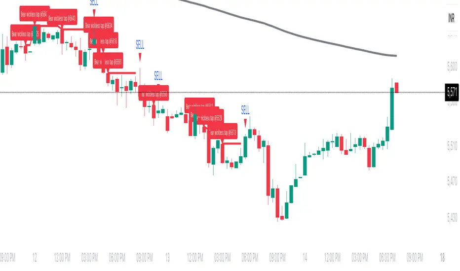
Advanced Market TheoryADVANCED MARKET THEORY (AMT)
This is not an indicator. It is a lens through which to see the true nature of the market.
Welcome to the definitive application of Auction Market Theory. What you have before you is the culmination of decades of market theory, fused with state-of-the-art data analysis and visual engineering. It is an institutional-grade intelligence engine designed for the serious trader who seeks to move beyond simplistic indicators and understand the fundamental forces that drive price.
This guide is your complete reference. Read it. Study it. Internalize it. The market is a complex story, and this tool is the language with which to read it.
PART I: THE GRAND THEORY - A UNIVERSE IN AN AUCTION
To understand the market, you must first understand its purpose. The market is a mechanism of discovery, organized by a continuous, two-way auction.
This foundational concept was pioneered by the legendary trader J. Peter Steidlmayer at the Chicago Board of Trade in the 1980s. He observed that beneath the chaotic facade of ticking prices lies a beautifully organized structure. The market's primary function is not to go up or down, but to facilitate trade by seeking a price level that encourages the maximum amount of interaction between buyers and sellers. This price is "value."
The Organizing Principle: The Normal Distribution
Over any given period, the market's activity will naturally form a bell curve (a normal distribution) turned on its side. This is the blueprint of the auction.
The Point of Control (POC): This is the peak of the bell curve—the single price level where the most trade occurred. It represents the point of maximum consensus, the "fairest price" as determined by the market participants. It is the gravitational center of the session.
The Value Area (VA): This is the heart of the bell curve, typically containing 70% of the session's activity (one standard deviation). This is the zone of "accepted value." Prices within this area are considered fair and are where the market is most comfortable conducting business.
The Extremes: The thin areas at the top and bottom of the curve are the "unfair" prices. These are levels where one side of the auction (buyers at the top, sellers at the bottom) was shut off, and trade was quickly rejected. These are areas of emotional trading and excess.
The Narrative of the Day: Balance vs. Imbalance
Every trading session is a story of the market's search for value.
Balance: When the market rotates and builds a symmetrical, bell-shaped profile, it is in a state of balance . Buyers and sellers are in agreement, and the market is range-bound.
Imbalance: When the market moves decisively away from a balanced area, it is in a state of imbalance . This is a trend. The market is actively seeking new information and a new area of value because the old one was rejected.
Your Purpose as a Trader
Your job is to read this story in real-time. Are we in balance or imbalance? Is the auction succeeding or failing at these new prices? The Advanced Market Theory engine is your Rosetta Stone to translate this complex narrative into actionable intelligence.
PART II: THE AMT ENGINE - AN EVOLUTION IN MARKET VISION
A standard market profile tool shows you a picture. The AMT Engine gives you the architect's full schematics, the engineer's stress tests, and the psychologist's behavioral analysis, all at once.
This is what makes it the Advanced Market Theory. We have fused the timeless principles with layers of modern intelligence:
TRINITY ANALYSIS: You can view the market through three distinct lenses. A Volume Profile shows where the money traded. A TPO (Time) Profile shows where the market spent its time. The revolutionary Hybrid Profile fuses both, giving you a complete picture of market conviction—marrying volume with duration.
AUTOMATED STRUCTURAL DECODING: The engine acts as your automated analyst, identifying critical structural phenomena in real-time:
Poor Highs/Lows: Weak auction points that signal a high probability of reversal.
Single Prints & Ledges: Footprints of rapid, aggressive market moves and areas of strong institutional acceptance.
Day Type Classification: The engine analyzes the session's personality as it develops ("Trend Day," "Normal Day," etc.), allowing you to adapt your strategy to the market's current character.
MACRO & MICRO FUSION: Via the Composite Profile , the engine merges weeks of data to reveal the major institutional battlegrounds that govern long-term price action. You can see the daily skirmish and the multi-month war on a single chart.
ORDER FLOW INTELLIGENCE: The ultimate advancement is the integrated Cumulative Volume Delta (CVD) engine. This moves beyond structure to analyze the raw aggression of buyers versus sellers. It is your window into the market's soul, automatically detecting critical Divergences that often precede major trend shifts.
ADAPTIVE SIGNALING: The engine's signal generation is not static; it is a thinking system. It evaluates setups based on a multi-factor Confluence Score , understands the market Regime (e.g., High Volatility), and adjusts its own confidence ( Probability % ) based on the complete context.
This is not a tool that gives you signals. This is a tool that gives you understanding .
PART III: THE VISUAL KEY - A LEXICON OF MARKET STRUCTURE
Every element on your chart is a piece of information. This is your guide to reading it fluently.
--- THE CORE ARCHITECTURE ---
The Profile Histogram: The primary visual on the left of each session. Its shape is the story. A thin profile is a trend; a fat, symmetrical profile is balance.
Blue Box : The zone of accepted, "fair" value. The heart of the session's business.
Bright Orange Line & Label : The Point of Control. The gravitational center. The price of maximum consensus. The most significant intraday level.
Dashed Blue Lines & Labels : The boundaries of value. Critical inflection points where the market decides to either remain in balance or seek value elsewhere.
Dashed Cyan Lines & Labels : The major, long-term structural levels derived from weeks of data. These are institutional reference points and carry immense weight. Treat them as primary support and resistance.
Dashed Orange Lines & Labels : Marks a Poor or Unfinished Auction . These represent emotional, weak extremes and are high-probability targets for future price action.
Diamond Markers : Mark Single Prints , which are footprints of aggressive, one-sided moves that left a "liquidity vacuum." Price is often drawn back to these levels to "repair" the poor structure.
Arrow Markers : Mark Ledges , which are areas of strong horizontal acceptance. They often act as powerful support/resistance in the future.
Dotted Gray Lines & Labels : The projected daily range based on multiples of the Initial Balance . Use them to set realistic profit targets and gauge the day's potential.
--- THE SIGNAL SUITE ---
Colored Triangles : These are your high-probability entry signals. The color is a strategic playbook:
Gold Triangle : ELITE Signal. An A+ setup with overwhelming confluence. This is the highest quality signal the engine can produce.
Yellow Triangle : FADE Signal. A counter-trend setup against an exhausted move at a structural extreme.
Cyan Triangle : BREAKOUT Signal. A momentum setup attempting to capitalize on a breakout from the value area.
Purple Triangle : ROTATION Signal. A mean-reversion setup within the value area, typically from one edge towards the POC.
Magenta Triangle : LIQUIDITY Signal. A sophisticated setup that identifies a "stop run" or liquidity sweep.
Percentage Number: The engine's calculated probability of success . This is not a guarantee, but a data-driven confidence score.
Dotted Gray Line: The signal's Entry Price .
Dashed Green Lines: The calculated Take Profit Targets .
Dashed Red Line: The calculated Stop Loss level.
PART IV: THE DASHBOARD - YOUR STRATEGIC COMMAND CENTER
The dashboard is your real-time intelligence briefing. It synthesizes all the engine's analysis into a clear, concise, and constantly updating summary.
--- CURRENT SESSION ---
POC, VAH, VAL: The live values for the core structure.
Profile Shape: Is the current auction top-heavy ( b-shaped ), bottom-heavy ( P-shaped ), or balanced ( D-shaped )?
VA Width: Is the value area expanding (trending) or contracting (balancing)?
Day Type: The engine's judgment on the day's personality. Use this to select the right strategy.
IB Range & POC Trend: Key metrics for understanding the opening sentiment and its evolution.
--- CVD ANALYSIS ---
Session CVD: The raw order flow. Is there more net buying or selling pressure in this session?
CVD Trend & DIVERGENCE: This is your order flow intelligence. Is the order flow confirming the price action? If "DIVERGENCE" flashes, it is a critical, high-alert warning of a potential reversal.
--- MARKET METRICS ---
Volume, ATR, RSI: Your standard contextual metrics, providing a quick read on activity, volatility, and momentum.
Regime: The engine's assessment of the broad market environment: High Volatility (favor breakouts), Low Volatility (favor mean reversion), or Normal .
--- PROFILE STATS, COMPOSITE, & STRUCTURE ---
These sections give you a quick quantitative summary of the profile structure, the major long-term Composite levels, and any active Poor Structures.
--- SIGNAL TYPES & ACTIVE SIGNAL ---
A permanent key to the signal colors and their meanings, along with the full details of the most recent active signal: its Type , Probability , Entry , Stop , and Target .
PART V: THE INPUTS MENU - CALIBRATING YOUR LENS
This engine is designed to be calibrated to your specific needs as a trader. Every input is a lever. This is not a "one size fits all" tool. The extensive tooltips are your built-in user manual, but here are the key areas of focus:
--- MARKET PROFILE ENGINE ---
Profile Mode: This is the most fundamental choice. Volume is the standard for price-based support and resistance. TPO is for analyzing time-based acceptance. Hybrid is the professional's choice, fusing both for a complete picture.
Profile Resolution: This is your zoom lens. Lower values for scalping and intraday precision. Higher values for a cleaner, big-picture view suitable for swing trading.
Composite Sessions: Your timeframe for macro analysis. 5-10 sessions for a weekly view; 20-30 sessions for a monthly, structural view.
--- SESSION & VALUE AREA ---
These settings must be configured correctly for your specific asset. The Session times are critical. The Initial Balance should reflect the key opening period for your market (60 minutes is standard for equities).
--- SIGNAL ENGINE & RISK MANAGEMENT ---
Signal Mode: THIS IS YOUR PERSONAL RISK PROFILE. Set it to Conservative to see only the absolute best A+ setups. Use Elite or Balanced for a standard approach. Use Aggressive only if you are an experienced scalper comfortable with managing more frequent, lower-probability setups.
ATR Multipliers: This suite gives you full, dynamic control over your risk/reward parameters. You can precisely define your initial stop loss distance and profit targets based on the market's current volatility.
A FINAL WORD FROM THE ARCHITECT
The creation of this engine was a journey into the very heart of market dynamics. It was born from a frustrating truth: that the most profound market theories were often confined to books and expensive institutional platforms, inaccessible to the modern retail trader. The goal was to bridge that gap.
The challenge was monumental. Making each discrete system—the volume profile, the TPO counter, the composite engine, the CVD tracker, the signal generator, the dynamic dashboard—work was a task in itself. But the true struggle, the frustrating, painstaking process that consumed countless hours, was making them work in unison . It was about ensuring the CVD analysis could intelligently inform the signal engine, that the day type classification could adjust the probability scores, and that the composite levels could provide context to the intraday structure, all in a seamless, real-time dance of data.
This engine is the result of that relentless pursuit of integration. It is built on the belief that a trader's greatest asset is not a signal, but clarity . It was designed to clear the noise, to organize the chaos, and to present the elegant, underlying logic of the market auction so that you can make better, more informed, and more confident decisions.
It is now in your hands. Use it not as a crutch, but as a lens. See the market for what it truly is.
"The market can remain irrational longer than you can remain solvent."
- John Maynard Keynes
DISCLAIMER
This script is an advanced analytical tool provided for informational and educational purposes only. It is not financial advice. All trading involves substantial risk, and past performance is not indicative of future results. The signals, probabilities, and metrics generated by this indicator do not constitute a recommendation to buy or sell any financial instrument. You, the user, are solely responsible for all trading decisions, risk management, and outcomes. Use this tool to supplement your own analysis and trading strategy.
PUBLISHING CATEGORIES
Volume Profile
Market Profile
Order Flow
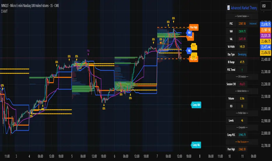
Correlation HeatMap [TradingFinder] Sessions Data Science Stats🔵 Introduction
n financial markets, correlation describes the statistical relationship between the price movements of two assets and how they interact over time. It plays a key role in both trading and investing by helping analyze asset behavior, manage portfolio risk, and understand intermarket dynamics. The Correlation Heatmap is a visual tool that shows how the correlation between multiple assets and a central reference asset (the Main Symbol) changes over time.
It supports four market types forex, stocks, crypto, and a custom mode making it adaptable to different trading environments. The heatmap uses a color-coded grid where warmer tones represent stronger negative correlations and cooler tones indicate stronger positive ones. This intuitive color system allows traders to quickly identify when assets move together or diverge, offering real-time insights that go beyond traditional correlation tables.
🟣 How to Interpret the Heatmap Visually ?
Each cell represents the correlation between the main symbol and one compared asset at a specific time.
Warm colors (e.g. red, orange) suggest strong negative correlation as one asset rises, the other tends to fall.
Cool colors (e.g. blue, green) suggest strong positive correlation both assets tend to move in the same direction.
Lighter shades indicate weaker correlations, while darker shades indicate stronger correlations.
The heatmap updates over time, allowing users to detect changes in correlation during market events or trading sessions.
One of the standout features of this indicator is its ability to overlay global market sessions such as Tokyo, London, New York, or major equity opens directly onto the heatmap timeline. This alignment lets traders observe how correlation structures respond to real-world session changes. For example, they can spot when assets shift from being inversely correlated to moving together as a new session opens, potentially signaling new momentum or macro flow. The customizable symbol setup (including up to 20 compared assets) makes it ideal not only for forex and crypto traders but also for multi-asset and sector-based stock analysis.
🟣 Use Cases and Advantages
Analyze sector rotation in equities by tracking correlation to major indices like SPX or DJI.
Monitor altcoin behavior relative to Bitcoin to find early entry opportunities in crypto markets.
Detect changes in currency alignment with DXY across trading sessions in forex.
Identify correlation breakdowns during market volatility, signaling possible new trends.
Use correlation shifts as confirmation for trade setups or to hedge multi-asset exposure
🔵 How to Use
Correlation is one of the core concepts in financial analysis and allows traders to understand how assets behave in relation to one another. The Correlation Heatmap extends this idea by going beyond a simple number or static matrix. Instead, it presents a dynamic visual map of how correlations shift over time.
In this indicator, a Main Symbol is selected as the reference point for analysis. In standard modes such as forex, stocks, or crypto, the symbol currently shown on the main chart is automatically used as the main symbol. This allows users to begin correlation analysis right away without adjusting any settings.
The horizontal axis of the heatmap shows time, while the vertical axis lists the selected assets. Each cell on the heatmap shows the correlation between that asset and the main symbol at a given moment.
This approach is especially useful for intermarket analysis. In forex, for example, tracking how currency pairs like OANDA:EURUSD EURUSD, FX:GBPUSD GBPUSD, and PEPPERSTONE:AUDUSD AUDUSD correlate with TVC:DXY DXY can give insight into broader capital flow.
If these pairs start showing increasing positive correlation with DXY say, shifting from blue to light green it could signal the start of a new phase or reversal. Conversely, if negative correlation fades gradually, it may suggest weakening relationships and more independent or volatile movement.
In the crypto market, watching how altcoins correlate with Bitcoin can help identify ideal entry points in secondary assets. In the stock market, analyzing how companies within the same sector move in relation to a major index like SP:SPX SPX or DJ:DJI DJI is also a highly effective technique for both technical and fundamental analysts.
This indicator not only visualizes correlation but also displays major market sessions. When enabled, this feature helps traders observe how correlation behavior changes at the start of each session, whether it's Tokyo, London, New York, or the opening of stock exchanges. Many key shifts, breakouts, or reversals tend to happen around these times, and the heatmap makes them easy to spot.
Another important feature is the market selection mode. Users can switch between forex, crypto, stocks, or custom markets and see correlation behavior specific to each one. In custom mode, users can manually select any combination of symbols for more advanced or personalized analysis. This makes the heatmap valuable not only for forex traders but also for stock traders, crypto analysts, and multi-asset strategists.
Finally, the heatmap's color-coded design helps users make sense of the data quickly. Warm colors such as red and orange reflect stronger negative correlations, while cool colors like blue and green represent stronger positive relationships. This simplicity and clarity make the tool accessible to both beginners and experienced traders.
🔵 Settings
Correlation Period: Allows you to set how many historical bars are used for calculating correlation. A higher number means a smoother, slower-moving heatmap, while a lower number makes it more responsive to recent changes.
Select Market: Lets you choose between Forex, Stock, Crypto, or Custom. In the first three options, the chart’s active symbol is automatically used as the Main Symbol. In Custom mode, you can manually define the Main Symbol and up to 20 Compared Symbols.
Show Open Session: Enables the display of major trading sessions such as Tokyo, London, New York, or equity market opening hours directly on the timeline. This helps you connect correlation shifts with real-world market activity.
Market Mode: Lets you select whether the displayed sessions relate to the forex or stock market.
🔵 Conclusion
The Correlation Heatmap is a robust and flexible tool for analyzing the relationship between assets across different markets. By tracking how correlations change in real time, traders can better identify alignment or divergence between symbols and gain valuable insights into market structure.
Support for multiple asset classes, session overlays, and intuitive visual cues make this one of the most effective tools for intermarket analysis.
Whether you’re looking to manage portfolio risk, validate entry points, or simply understand capital flow across markets, this heatmap provides a clear and actionable perspective that you can rely on.

BE-Indicator Aggregator toolkit█ Overview:
BE-Indicator Aggregator toolkit is a toolkit which is built for those we rely on taking multi-confirmation from different indicators available with the traders. This Toolkit aid's traders in understanding their custom logic for their trade setups and provides the summarized results on how it performed over the past.
█ How It Works:
Load the external indicator plots in the indicator input setting
Provide your custom logic for the trade setup
Set your expected SL & TP values
█ Legends, Definitions & Logic Building Rules:
Building the logic for your trade setup plays a pivotal role in the toolkit, it shall be broken into parts and toolkit aims to understand each of the logical parts of your setup and interpret the outcome as trade accuracy.
Toolkit broadly aims to understand 4 types of inputs in "Condition Builder"
Comments : Line which starts with single quotation ( ' ) shall be ignored by toolkit while understanding the logic.
Note: Blank line space or less than 3 characters are treated equally to comments.
Long Condition: Line which starts with " L- " shall be considered for identifying Long setups.
Short Condition: Line which starts with " S- " shall be considered for identifying Short setups.
Variables: Line which starts with " VAR- " shall be considered as variables. Variables can be one such criteria for Long or short condition.
Building Rules: Define all variables first then specify the condition. The usual declare and assign concept of programming. :p)
Criteria Rules: Criteria are individual logic for your one parent condition. multiple criteria can be present in one condition. Each parameter should be delimited with ' | ' key and each criteria should be delimited with ' , ' (Comma with a space - IMPORTANT!!!)
█ Sample Codes for Conditional Builder:
For Trading Long when Open = Low
For Trading Short when Open = High with a Red candle
'Long Setup <---- Comment
L-O|E|L
' E <- in the above line refers to Equals ' = '
'Short Setup
S-AND:O|E|H, O|G|C
' 2 Criteria for used building one condition. Since, both have to satisfied used "AND:" logic.
Understanding of Operator Legends:
"E" => Refers to Equals
"NE" => Refers to Not Equals
"NEOR" => Logical value is Either Comparing value 1 or Comparing value 2
"NEAND" => Logical value is Comparing value 1 And Comparing value 2
"G" => Logical value Greater than Comparing value 1
"GE" => Logical value Greater than and equal to Comparing value 1
"L" => Logical value Lesser than Comparing value 1
"LE" => Logical value Lesser than and equal to Comparing value 1
"B" => Logical value is Between Comparing value 1 & Comparing value 2
"BE" => Logical value is Between or Equal to Comparing value 1 & Comparing value 2
"OSE" => Logical value is Outside of Comparing value 1 & Comparing value 2
"OSI" => Logical value is Outside or Equal to Comparing value 1 & Comparing value 2
"ERR" => Logical value is 'na'
"NERR" => Logical value is not 'na'
"CO" => Logical value Crossed Over Comparing value 1
"CU" => Logical value Crossed Under Comparing value 1
Understanding of Condition Legends:
AND: -> All criteria's to be satisfied for the condition to be True.
NAND: -> Output of AND condition shall be Inversed for the condition to be True.
OR: -> One of criteria to be satisfied for the condition to be True.
NOR: -> Output of OR condition shall be Inversed for the condition to be True.
ATLEAST:X: -> At-least X no of criteria to be satisfied for the condition to be True.
Note: "X" can be any number
NATLEAST:X: -> Output of ATLEAST condition shall be Inversed for the condition to be True
WASTRUE:X: -> Single criteria WAS TRUE within X bar in past for the condition to be True.
Note: "X" can be any number.
ISTRUE:X: -> Single criteria is TRUE since X bar in past for the condition to be True.
Note: "X" can be any number.
Understanding of Variable Legends:
While Condition Supports 8 Types, Variable supports only 6 Types listed below
AND: -> All criteria's to be satisfied for the Variable to be True.
NAND: -> Output of AND condition shall be Inversed for the Variable to be True.
OR: -> One of criteria to be satisfied for the Variable to be True.
NOR: -> Output of OR condition shall be Inversed for the Variable to be True.
ATLEAST:X: -> At-least X no of criteria to be satisfied for the Variable to be True.
Note: "X" can be any number
NATLEAST:X: -> Output of ATLEAST condition shall be Inversed for the Variable to be True
█ Sample Outputs with Logics:
1. RSI Indicator + Technical Indicator: StopLoss: 2.25 against Reward ratio of 1.75 (3.94 value)
Plots Used in Indicator Settings:
Source 1:- RSI
Source 2:- RSI Based MA
Source 3:- Strong Buy
Source 4:- Strong Sell
Logic Used:
For Long Setup : RSI Should be above RSI Based MA, RSI has been Rising when compared to 3 candles ago, Technical Indicator signaled for a Strong Buy on the current candle, however in last 6 candles Technical indicator signaled for Strong Sell.
Similarly Inverse for Short Setup.
L-AND:ES1|GE|ES2, ES1|G|ES1
L-ES3|E|1
L-OR:ES4 |E|1, ES4 |E|1, ES4 |E|1, ES4 |E|1, ES4 |E|1, ES4 |E|1
S-AND:ES1|LE|ES2, ES1|L|ES1
S-ES4|E|1
S-OR:ES3 |E|1, ES3 |E|1, ES3 |E|1, ES3 |E|1, ES3 |E|1, ES3 |E|1
'Note: Last OR condition can also be written by using WASTRUE definition like below
'L-WASTRUE:6:ES4|E|1
'S-WASTRUE:6:ES3|E|1
Output:
2. Volumatic Support / Resistance Levels :
Plots Used in Indicator Settings:
Source 1:- Resistance
Source 2:- Support
Logic Used:
For Long Setup : Long Trade on Liquidity Support.
For Short Setup : Short Trade on Liquidity Resistance.
'Variable Named "ChkLowTradingAbvSupport" is declared to check if last 3 candles is trading above support line of liquidity.
VAR-ChkLowTradingAbvSupport:AND:L|G|ES2, L |G|ES2, L |G|ES2
'Variable Named "ChkCurBarClsdAbv4thBarHigh" is declared to check if current bar closed above the high of previous candle where the Liquidity support is taken (4th Bar).
VAR-ChkCurBarClsdAbv4thBarHigh:OR:C|GE|H , L|G|H
'Combining Condition and Variable to Initiate Long Trade Logic
L-L |LE|ES2
L-AND:ChkLowTradingAbvSupport, ChkCurBarClsdAbv4thBarHigh
VAR-ChkHghTradingBlwRes:AND:H|L|ES1, H |L|ES1, H |L|ES1
VAR-ChkCurBarClsdBlw4thBarLow:OR:C|LE|L , H|L|L
S-H |GE|ES1
S-AND:ChkHghTradingBlwRes, ChkCurBarClsdBlw4thBarLow
Output 1: Day Trading Version
Output 2: Scalper Version
Output 3: Position Version

DrawZigZag🟩 OVERVIEW
This library draws zigzag lines for existing pivots. It is designed to be simple to use. If your script creates pivots and you want to join them up while handling edge cases, this library does that quickly and efficiently. If you want your pivots created for you, choose one of the many other zigzag libraries that do that.
🟩 HOW TO USE
Pine Script libraries contain reusable code for importing into indicators. You do not need to copy any code out of here. Just import the library and call the function you want.
For example, for version 1 of this library, import it like this:
import SimpleCryptoLife/DrawZigZag/1
See the EXAMPLE USAGE sections within the library for examples of calling the functions.
For more information on libraries and incorporating them into your scripts, see the Libraries section of the Pine Script User Manual.
🟩 WHAT IT DOES
I looked at every zigzag library on TradingView, after finishing this one. They all seemed to fall into two groups in terms of functionality:
• Create the pivots themselves, using a combination of Williams-style pivots and sometimes price distance.
• Require an array of pivot information, often in a format that uses user-defined types.
My library takes a completely different approach.
Firstly, it only does the drawing. It doesn't calculate the pivots for you. This isn't laziness. There are so many ways to define pivots and that should be up to you. If you've followed my work on market structure you know what I think of Williams pivots.
Secondly, when you pass information about your pivots to the library function, you only need the minimum of pivot information -- whether it's a High or Low pivot, the price, and the bar index. Pass these as normal variables -- bools, ints, and floats -- on the fly as your pivots confirm. It is completely agnostic as to how you derive your pivots. If they are confirmed an arbitrary number of bars after they happen, that's fine.
So why even bother using it if all it does it draw some lines?
Turns out there is quite some logic needed in order to connect highs and lows in the right way, and to handle edge cases. This is the kind of thing one can happily outsource.
🟩 THE RULES
• Zigs and zags must alternate between Highs and Lows. We never connect a High to a High or a Low to a Low.
• If a candle has both a High and Low pivot confirmed on it, the first line is drawn to the end of the candle that is the opposite to the previous pivot. Then the next line goes vertically through the candle to the other end, and then after that continues normally.
• If we draw a line up from a Low to a High pivot, and another High pivot comes in higher, we *extend* the line up, and the same for lines down. Yes this is a form of repainting. It is in my opinion the only way to end up with a correct structure.
• We ignore lower highs on the way up and higher lows on the way down.
🟩 WHAT'S COOL ABOUT THIS LIBRARY
• It's simple and lightweight: no exported user-defined types, no helper methods, no matrices.
• It's really fast. In my profiling it runs at about ~50ms, and changing the options (e.g., trimming the array) doesn't make very much difference.
• You only need to call one function, which does all the calculations and draws all lines.
• There are two variations of this function though -- one simple function that just draws lines, and one slightly more advanced method that modifies an array containing the lines. If you don't know which one you want, use the simpler one.
🟩 GEEK STUFF
• There are no dependencies on other libraries.
• I tried to make the logic as clear as I could and comment it appropriately.
• In the `f_drawZigZags` function, the line variable is declared using the `var` keyword *inside* the function, for simplicity. For this reason, it persists between function calls *only* if the function is called from the global scope or a local if block. In general, if a function is called from inside a loop , or multiple times from different contexts, persistent variables inside that function are re-initialised on each call. In this case, this re-initialisation would mean that the function loses track of the previous line, resulting in incorrect drawings. This is why you cannot call the `f_drawZigZags` function from a loop (not that there's any reason to). The `m_drawZigZagsArray` does not use any internal `var` variables.
• The function itself takes a Boolean parameter `_showZigZag`, which turns the drawings on and off, so there is no need to call the function conditionally. In the examples, we do call the functions from an if block, purely as an illustration of how to increase performance by restricting the amount of code that needs to be run.
🟩 BRING ON THE FUNCTIONS
f_drawZigZags(_showZigZag, _isHighPivot, _isLowPivot, _highPivotPrice, _lowPivotPrice, _pivotIndex, _zigzagWidth, _lineStyle, _upZigColour, _downZagColour)
This function creates or extends the latest zigzag line. Takes real-time information about pivots and draws lines. It does not calculate the pivots. It must be called once per script and cannot be called from a loop.
Parameters:
_showZigZag (bool) : Whether to show the zigzag lines.
_isHighPivot (bool) : Whether the current bar confirms a high pivot. Note that pivots are confirmed after the bar in which they occur.
_isLowPivot (bool) : Whether the current bar confirms a low pivot.
_highPivotPrice (float) : The price of the high pivot that was confirmed this bar. It is NOT the high price of the current bar.
_lowPivotPrice (float) : The price of the low pivot that was confirmed this bar. It is NOT the low price of the current bar.
_pivotIndex (int) : The bar index of the pivot that was confirmed this bar. This is not an offset. It's the `bar_index` value of the pivot.
_zigzagWidth (int) : The width of the zigzag lines.
_lineStyle (string) : The style of the zigzag lines.
_upZigColour (color) : The colour of the up zigzag lines.
_downZagColour (color) : The colour of the down zigzag lines.
Returns: The function has no explicit returns. As a side effect, it draws or updates zigzag lines.
method m_drawZigZagsArray(_a_zigZagLines, _showZigZag, _isHighPivot, _isLowPivot, _highPivotPrice, _lowPivotPrice, _pivotIndex, _zigzagWidth, _lineStyle, _upZigColour, _downZagColour, _trimArray)
Namespace types: array
Parameters:
_a_zigZagLines (array)
_showZigZag (bool) : Whether to show the zigzag lines.
_isHighPivot (bool) : Whether the current bar confirms a high pivot. Note that pivots are usually confirmed after the bar in which they occur.
_isLowPivot (bool) : Whether the current bar confirms a low pivot.
_highPivotPrice (float) : The price of the high pivot that was confirmed this bar. It is NOT the high price of the current bar.
_lowPivotPrice (float) : The price of the low pivot that was confirmed this bar. It is NOT the low price of the current bar.
_pivotIndex (int) : The bar index of the pivot that was confirmed this bar. This is not an offset. It's the `bar_index` value of the pivot.
_zigzagWidth (int) : The width of the zigzag lines.
_lineStyle (string) : The style of the zigzag lines.
_upZigColour (color) : The colour of the up zigzag lines.
_downZagColour (color) : The colour of the down zigzag lines.
_trimArray (bool) : If true, the array of lines is kept to a maximum size of two lines (the line elements are not deleted). If false (the default), the array is kept to a maximum of 500 lines (the maximum number of line objects a single Pine script can display).
Returns: This function has no explicit returns but it modifies a global array of zigzag lines.
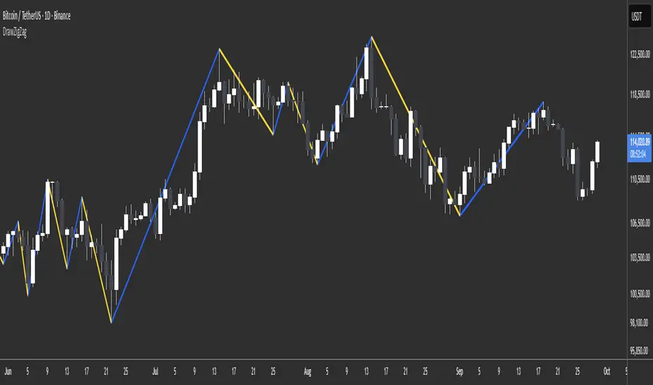
Market Zone Analyzer[BullByte]Understanding the Market Zone Analyzer
---
1. Purpose of the Indicator
The Market Zone Analyzer is a Pine Script™ (version 6) indicator designed to streamline market analysis on TradingView. Rather than scanning multiple separate tools, it unifies four core dimensions—trend strength, momentum, price action, and market activity—into a single, consolidated view. By doing so, it helps traders:
• Save time by avoiding manual cross-referencing of disparate signals.
• Reduce decision-making errors that can arise from juggling multiple indicators.
• Gain a clear, reliable read on whether the market is in a bullish, bearish, or sideways phase, so they can more confidently decide to enter, exit, or hold a position.
---
2. Why a Trader Should Use It
• Unified View: Combines all essential market dimensions into one easy-to-read score and dashboard, eliminating the need to piece together signals manually.
• Adaptability: Automatically adjusts its internal weighting for trend, momentum, and price action based on current volatility. Whether markets are choppy or calm, the indicator remains relevant.
• Ease of Interpretation: Outputs a simple “BULLISH,” “BEARISH,” or “SIDEWAYS” label, supplemented by an intuitive on-chart dashboard and an oscillator plot that visually highlights market direction.
• Reliability Features: Built-in smoothing of the net score and hysteresis logic (requiring consecutive confirmations before flips) minimize false signals during noisy or range-bound phases.
---
3. Why These Specific Indicators?
This script relies on a curated set of well-established technical tools, each chosen for its particular strength in measuring one of the four core dimensions:
1. Trend Strength:
• ADX/DMI (Average Directional Index / Directional Movement Index): Measures how strong a trend is, and whether the +DI line is above the –DI line (bullish) or vice versa (bearish).
• Moving Average Slope (Fast MA vs. Slow MA): Compares a shorter-period SMA to a longer-period SMA; if the fast MA sits above the slow MA, it confirms an uptrend, and vice versa for a downtrend.
• Ichimoku Cloud Differential (Senkou A vs. Senkou B): Provides a forward-looking view of trend direction; Senkou A above Senkou B signals bullishness, and the opposite signals bearishness.
2. Momentum:
• Relative Strength Index (RSI): Identifies overbought (above its dynamically calculated upper bound) or oversold (below its lower bound) conditions; changes in RSI often precede price reversals.
• Stochastic %K: Highlights shifts in short-term momentum by comparing closing price to the recent high/low range; values above its upper band signal bullish momentum, below its lower band signal bearish momentum.
• MACD Histogram: Measures the difference between the MACD line and its signal line; a positive histogram indicates upward momentum, a negative histogram indicates downward momentum.
3. Price Action:
• Highest High / Lowest Low (HH/LL) Range: Over a defined lookback period, this captures breakout or breakdown levels. A closing price near the recent highs (with a positive MA slope) yields a bullish score, and near the lows (with a negative MA slope) yields a bearish score.
• Heikin-Ashi Doji Detection: Uses Heikin-Ashi candles to identify indecision or continuation patterns. A small Heikin-Ashi body (doji) relative to recent volatility is scored as neutral; a larger body in the direction of the MA slope is scored bullish or bearish.
• Candle Range Measurement: Compares each candle’s high-low range against its own dynamic band (average range ± standard deviation). Large candles aligning with the prevailing trend score bullish or bearish accordingly; unusually small candles can indicate exhaustion or consolidation.
4. Market Activity:
• Bollinger Bands Width (BBW): Measures the distance between BB upper and lower bands; wide bands indicate high volatility, narrow bands indicate low volatility.
• Average True Range (ATR): Quantifies average price movement (volatility). A sudden spike in ATR suggests a volatile environment, while a contraction suggests calm.
• Keltner Channels Width (KCW): Similar to BBW but uses ATR around an EMA. Provides a second layer of volatility context, confirming or contrasting BBW readings.
• Volume (with Moving Average): Compares current volume to its moving average ± standard deviation. High volume validates strong moves; low volume signals potential lack of conviction.
By combining these tools, the indicator captures trend direction, momentum strength, price-action nuances, and overall market energy, yielding a more balanced and comprehensive assessment than any single tool alone.
---
4. What Makes This Indicator Stand Out
• Multi-Dimensional Analysis: Rather than relying on a lone oscillator or moving average crossover, it simultaneously evaluates trend, momentum, price action, and activity.
• Dynamic Weighting: The relative importance of trend, momentum, and price action adjusts automatically based on real-time volatility (Market Activity State). For example, in highly volatile conditions, trend and momentum signals carry more weight; in calm markets, price action signals are prioritized.
• Stability Mechanisms:
• Smoothing: The net score is passed through a short moving average, filtering out noise, especially on lower timeframes.
• Hysteresis: Both Market Activity State and the final bullish/bearish/sideways zone require two consecutive confirmations before flipping, reducing whipsaw.
• Visual Interpretation: A fully customizable on-chart dashboard displays each sub-indicator’s value, regime, score, and comment, all color-coded. The oscillator plot changes color to reflect the current market zone (green for bullish, red for bearish, gray for sideways) and shows horizontal threshold lines at +2, 0, and –2.
---
5. Recommended Timeframes
• Short-Term (5 min, 15 min): Day traders and scalpers can benefit from rapid signals, but should enable smoothing (and possibly disable hysteresis) to reduce false whipsaws.
• Medium-Term (1 h, 4 h): Swing traders find a balance between responsiveness and reliability. Less smoothing is required here, and the default parameters (e.g., ADX length = 14, RSI length = 14) perform well.
• Long-Term (Daily, Weekly): Position traders tracking major trends can disable smoothing for immediate raw readings, since higher-timeframe noise is minimal. Adjust lookback lengths (e.g., increase adxLength, rsiLength) if desired for slower signals.
Tip: If you keep smoothing off, stick to timeframes of 1 h or higher to avoid excessive signal “chatter.”
---
6. How Scoring Works
A. Individual Indicator Scores
Each sub-indicator is assigned one of three discrete scores:
• +1 if it indicates a bullish condition (e.g., RSI above its dynamically calculated upper bound).
• 0 if it is neutral (e.g., RSI between upper and lower bounds).
• –1 if it indicates a bearish condition (e.g., RSI below its dynamically calculated lower bound).
Examples of individual score assignments:
• ADX/DMI:
• +1 if ADX ≥ adxThreshold and +DI > –DI (strong bullish trend)
• –1 if ADX ≥ adxThreshold and –DI > +DI (strong bearish trend)
• 0 if ADX < adxThreshold (trend strength below threshold)
• RSI:
• +1 if RSI > RSI_upperBound
• –1 if RSI < RSI_lowerBound
• 0 otherwise
• ATR (as part of Market Activity):
• +1 if ATR > (ATR_MA + stdev(ATR))
• –1 if ATR < (ATR_MA – stdev(ATR))
• 0 otherwise
Each of the four main categories shares this same +1/0/–1 logic across their sub-components.
B. Category Scores
Once each sub-indicator reports +1, 0, or –1, these are summed within their categories as follows:
• Trend Score = (ADX score) + (MA slope score) + (Ichimoku differential score)
• Momentum Score = (RSI score) + (Stochastic %K score) + (MACD histogram score)
• Price Action Score = (Highest-High/Lowest-Low score) + (Heikin-Ashi doji score) + (Candle range score)
• Market Activity Raw Score = (BBW score) + (ATR score) + (KC width score) + (Volume score)
Each category’s summed value can range between –3 and +3 (for Trend, Momentum, and Price Action), and between –4 and +4 for Market Activity raw.
C. Market Activity State and Dynamic Weight Adjustments
Rather than contributing directly to the netScore like the other three categories, Market Activity determines how much weight to assign to Trend, Momentum, and Price Action:
1. Compute Market Activity Raw Score by summing BBW, ATR, KCW, and Volume individual scores (each +1/0/–1).
2. Bucket into High, Medium, or Low Activity:
• High if raw Score ≥ 2 (volatile market).
• Low if raw Score ≤ –2 (calm market).
• Medium otherwise.
3. Apply Hysteresis (if enabled): The state only flips after two consecutive bars register the same high/low/medium label.
4. Set Category Weights:
• High Activity: Trend = 50 %, Momentum = 35 %, Price Action = 15 %.
• Low Activity: Trend = 25 %, Momentum = 20 %, Price Action = 55 %.
• Medium Activity: Use the trader’s base weight inputs (e.g., Trend = 40 %, Momentum = 30 %, Price Action = 30 % by default).
D. Calculating the Net Score
5. Normalize Base Weights (so that the sum of Trend + Momentum + Price Action always equals 100 %).
6. Determine Current Weights based on the Market Activity State (High/Medium/Low).
7. Compute Each Category’s Contribution: Multiply (categoryScore) × (currentWeight).
8. Sum Contributions to get the raw netScore (a floating-point value that can exceed ±3 when scores are strong).
9. Smooth the netScore over two bars (if smoothing is enabled) to reduce noise.
10. Apply Hysteresis to the Final Zone:
• If the smoothed netScore ≥ +2, the bar is classified as “Bullish.”
• If the smoothed netScore ≤ –2, the bar is classified as “Bearish.”
• Otherwise, it is “Sideways.”
• To prevent rapid flips, the script requires two consecutive bars in the new zone before officially changing the displayed zone (if hysteresis is on).
E. Thresholds for Zone Classification
• BULLISH: netScore ≥ +2
• BEARISH: netScore ≤ –2
• SIDEWAYS: –2 < netScore < +2
---
7. Role of Volatility (Market Activity State) in Scoring
Volatility acts as a dynamic switch that shifts which category carries the most influence:
1. High Activity (Volatile):
• Detected when at least two sub-scores out of BBW, ATR, KCW, and Volume equal +1.
• The script sets Trend weight = 50 % and Momentum weight = 35 %. Price Action weight is minimized at 15 %.
• Rationale: In volatile markets, strong trending moves and momentum surges dominate, so those signals are more reliable than nuanced candle patterns.
2. Low Activity (Calm):
• Detected when at least two sub-scores out of BBW, ATR, KCW, and Volume equal –1.
• The script sets Price Action weight = 55 %, Trend = 25 %, and Momentum = 20 %.
• Rationale: In quiet, sideways markets, subtle price-action signals (breakouts, doji patterns, small-range candles) are often the best early indicators of a new move.
3. Medium Activity (Balanced):
• Raw Score between –1 and +1 from the four volatility metrics.
• Uses whatever base weights the trader has specified (e.g., Trend = 40 %, Momentum = 30 %, Price Action = 30 %).
Because volatility can fluctuate rapidly, the script employs hysteresis on Market Activity State: a new High or Low state must occur on two consecutive bars before weights actually shift. This avoids constant back-and-forth weight changes and provides more stability.
---
8. Scoring Example (Hypothetical Scenario)
• Symbol: Bitcoin on a 1-hour chart.
• Market Activity: Raw volatility sub-scores show BBW (+1), ATR (+1), KCW (0), Volume (+1) → Total raw Score = +3 → High Activity.
• Weights Selected: Trend = 50 %, Momentum = 35 %, Price Action = 15 %.
• Trend Signals:
• ADX strong and +DI > –DI → +1
• Fast MA above Slow MA → +1
• Ichimoku Senkou A > Senkou B → +1
→ Trend Score = +3
• Momentum Signals:
• RSI above upper bound → +1
• MACD histogram positive → +1
• Stochastic %K within neutral zone → 0
→ Momentum Score = +2
• Price Action Signals:
• Highest High/Lowest Low check yields 0 (close not near extremes)
• Heikin-Ashi doji reading is neutral → 0
• Candle range slightly above upper bound but trend is strong, so → +1
→ Price Action Score = +1
• Compute Net Score (before smoothing):
• Trend contribution = 3 × 0.50 = 1.50
• Momentum contribution = 2 × 0.35 = 0.70
• Price Action contribution = 1 × 0.15 = 0.15
• Raw netScore = 1.50 + 0.70 + 0.15 = 2.35
• Since 2.35 ≥ +2 and hysteresis is met, the final zone is “Bullish.”
Although the netScore lands at 2.35 (Bullish), smoothing might bring it slightly below 2.00 on the first bar (e.g., 1.90), in which case the script would wait for a second consecutive reading above +2 before officially classifying the zone as Bullish (if hysteresis is enabled).
---
9. Correlation Between Categories
The four categories—Trend Strength, Momentum, Price Action, and Market Activity—often reinforce or offset one another. The script takes advantage of these natural correlations:
• Bullish Alignment: If ADX is strong and pointed upward, fast MA is above slow MA, and Ichimoku is positive, that usually coincides with RSI climbing above its upper bound and the MACD histogram turning positive. In such cases, both Trend and Momentum categories generate +1 or +2. Because the Market Activity State is likely High (given the accompanying volatility), Trend and Momentum weights are at their peak, so the netScore quickly crosses into Bullish territory.
• Sideways/Consolidation: During a low-volatility, sideways phase, ADX may fall below its threshold, MAs may flatten, and RSI might hover in the neutral band. However, subtle price-action signals (like a small breakout candle or a Heikin-Ashi candle with a slight bias) can still produce a +1 in the Price Action category. If Market Activity is Low, Price Action’s weight (55 %) can carry enough influence—even if Trend and Momentum are neutral—to push the netScore out of “Sideways” into a mild bullish or bearish bias.
• Opposing Signals: When Trend is bullish but Momentum turns negative (for example, price continues up but RSI rolls over), the two scores can partially cancel. Market Activity may remain Medium, in which case the netScore lingers near zero (Sideways). The trader can then wait for either a clearer momentum shift or a fresh price-action breakout before committing.
By dynamically recognizing these correlations and adjusting weights, the indicator ensures that:
• When Trend and Momentum align (and volatility supports it), the netScore leaps strongly into Bullish or Bearish.
• When Trend is neutral but Price Action shows an early move in a low-volatility environment, Price Action’s extra weight in the Low Activity State can still produce actionable signals.
---
10. Market Activity State & Its Role (Detailed)
The Market Activity State is not a direct category score—it is an overarching context setter for how heavily to trust Trend, Momentum, or Price Action. Here’s how it is derived and applied:
1. Calculate Four Volatility Sub-Scores:
• BBW: Compare the current band width to its own moving average ± standard deviation. If BBW > (BBW_MA + stdev), assign +1 (high volatility); if BBW < (BBW_MA × 0.5), assign –1 (low volatility); else 0.
• ATR: Compare ATR to its moving average ± standard deviation. A spike above the upper threshold is +1; a contraction below the lower threshold is –1; otherwise 0.
• KCW: Same logic as ATR but around the KCW mean.
• Volume: Compare current volume to its volume MA ± standard deviation. Above the upper threshold is +1; below the lower threshold is –1; else 0.
2. Sum Sub-Scores → Raw Market Activity Score: Range between –4 and +4.
3. Assign Market Activity State:
• High Activity: Raw Score ≥ +2 (at least two volatility metrics are strongly spiking).
• Low Activity: Raw Score ≤ –2 (at least two metrics signal unusually low volatility or thin volume).
• Medium Activity: Raw Score is between –1 and +1 inclusive.
4. Hysteresis for Stability:
• If hysteresis is enabled, a new state only takes hold after two consecutive bars confirm the same High, Medium, or Low label.
• This prevents the Market Activity State from bouncing around when volatility is on the fence.
5. Set Category Weights Based on Activity State:
• High Activity: Trend = 50 %, Momentum = 35 %, Price Action = 15 %.
• Low Activity: Trend = 25 %, Momentum = 20 %, Price Action = 55 %.
• Medium Activity: Use trader’s base weights (e.g., Trend = 40 %, Momentum = 30 %, Price Action = 30 %).
6. Impact on netScore: Because category scores (–3 to +3) multiply by these weights, High Activity amplifies the effect of strong Trend and Momentum scores; Low Activity amplifies the effect of Price Action.
7. Market Context Tooltip: The dashboard includes a tooltip summarizing the current state—e.g., “High activity, trend and momentum prioritized,” “Low activity, price action prioritized,” or “Balanced market, all categories considered.”
---
11. Category Weights: Base vs. Dynamic
Traders begin by specifying base weights for Trend Strength, Momentum, and Price Action that sum to 100 %. These apply only when volatility is in the Medium band. Once volatility shifts:
• High Volatility Overrides:
• Trend jumps from its base (e.g., 40 %) to 50 %.
• Momentum jumps from its base (e.g., 30 %) to 35 %.
• Price Action is reduced to 15 %.
Example: If base weights were Trend = 40 %, Momentum = 30 %, Price Action = 30 %, then in High Activity they become 50/35/15. A Trend score of +3 now contributes 3 × 0.50 = +1.50 to netScore; a Momentum +2 contributes 2 × 0.35 = +0.70. In total, Trend + Momentum can easily push netScore above the +2 threshold on its own.
• Low Volatility Overrides:
• Price Action leaps from its base (30 %) to 55 %.
• Trend falls to 25 %, Momentum falls to 20 %.
Why? When markets are quiet, subtle candle breakouts, doji patterns, and small-range expansions tend to foreshadow the next swing more effectively than raw trend readings. A Price Action score of +3 in this state contributes 3 × 0.55 = +1.65, which can carry the netScore toward +2—even if Trend and Momentum are neutral or only mildly positive.
Because these weight shifts happen only after two consecutive bars confirm a High or Low state (if hysteresis is on), the indicator avoids constantly flipping its emphasis during borderline volatility phases.
---
12. Dominant Category Explained
Within the dashboard, a label such as “Trend Dominant,” “Momentum Dominant,” or “Price Action Dominant” appears when one category’s absolute weighted contribution to netScore is the largest. Concretely:
• Compute each category’s weighted contribution = (raw category score) × (current weight).
• Compare the absolute values of those three contributions.
• The category with the highest absolute value is flagged as Dominant for that bar.
Why It Matters:
• Momentum Dominant: Indicates that the combined force of RSI, Stochastic, and MACD (after weighting) is pushing netScore farther than either Trend or Price Action. In practice, it means that short-term sentiment and speed of change are the primary drivers right now, so traders should watch for continued momentum signals before committing to a trade.
• Trend Dominant: Means ADX, MA slope, and Ichimoku (once weighted) outweigh the other categories. This suggests a strong directional move is in place; trend-following entries or confirming pullbacks are likely to succeed.
• Price Action Dominant: Occurs when breakout/breakdown patterns, Heikin-Ashi candle readings, and range expansions (after weighting) are the most influential. This often happens in calmer markets, where subtle shifts in candle structure can foreshadow bigger moves.
By explicitly calling out which category is carrying the most weight at any moment, the dashboard gives traders immediate insight into why the netScore is tilting toward bullish, bearish, or sideways.
---
13. Oscillator Plot: How to Read It
The “Net Score” oscillator sits below the dashboard and visually displays the smoothed netScore as a line graph. Key features:
1. Value Range: In normal conditions it oscillates roughly between –3 and +3, but extreme confluences can push it outside that range.
2. Horizontal Threshold Lines:
• +2 Line (Bullish threshold)
• 0 Line (Neutral midline)
• –2 Line (Bearish threshold)
3. Zone Coloring:
• Green Background (Bullish Zone): When netScore ≥ +2.
• Red Background (Bearish Zone): When netScore ≤ –2.
• Gray Background (Sideways Zone): When –2 < netScore < +2.
4. Dynamic Line Color:
• The plotted netScore line itself is colored green in a Bullish Zone, red in a Bearish Zone, or gray in a Sideways Zone, creating an immediate visual cue.
Interpretation Tips:
• Crossing Above +2: Signals a strong enough combined trend/momentum/price-action reading to classify as Bullish. Many traders wait for a clear crossing plus a confirmation candle before entering a long position.
• Crossing Below –2: Indicates a strong Bearish signal. Traders may consider short or exit strategies.
• Rising Slope, Even Below +2: If netScore climbs steadily from neutral toward +2, it demonstrates building bullish momentum.
• Divergence: If price makes a higher high but the oscillator fails to reach a new high, it can warn of weakening momentum and a potential reversal.
---
14. Comments and Their Necessity
Every sub-indicator (ADX, MA slope, Ichimoku, RSI, Stochastic, MACD, HH/LL, Heikin-Ashi, Candle Range, BBW, ATR, KCW, Volume) generates a short comment that appears in the detailed dashboard. Examples:
• “Strong bullish trend” or “Strong bearish trend” for ADX/DMI
• “Fast MA above slow MA” or “Fast MA below slow MA” for MA slope
• “RSI above dynamic threshold” or “RSI below dynamic threshold” for RSI
• “MACD histogram positive” or “MACD histogram negative” for MACD Hist
• “Price near highs” or “Price near lows” for HH/LL checks
• “Bullish Heikin Ashi” or “Bearish Heikin Ashi” for HA Doji scoring
• “Large range, trend confirmed” or “Small range, trend contradicted” for Candle Range
Additionally, the top-row comment for each category is:
• Trend: “Highly Bullish,” “Highly Bearish,” or “Neutral Trend.”
• Momentum: “Strong Momentum,” “Weak Momentum,” or “Neutral Momentum.”
• Price Action: “Bullish Action,” “Bearish Action,” or “Neutral Action.”
• Market Activity: “Volatile Market,” “Calm Market,” or “Stable Market.”
Reasons for These Comments:
• Transparency: Shows exactly how each sub-indicator contributed to its category score.
• Education: Helps traders learn why a category is labeled bullish, bearish, or neutral, building intuition over time.
• Customization: If, for example, the RSI comment says “RSI neutral” despite an impending trend shift, a trader might choose to adjust RSI length or thresholds.
In the detailed dashboard, hovering over each comment cell also reveals a tooltip with additional context (e.g., “Fast MA above slow MA” or “Senkou A above Senkou B”), helping traders understand the precise rule behind that +1, 0, or –1 assignment.
---
15. Real-Life Example (Consolidated)
• Instrument & Timeframe: Bitcoin (BTCUSD), 1-hour chart.
• Current Market Activity: BBW and ATR both spike (+1 each), KCW is moderately high (+1), but volume is only neutral (0) → Raw Market Activity Score = +2 → State = High Activity (after two bars, if hysteresis is on).
• Category Weights Applied: Trend = 50 %, Momentum = 35 %, Price Action = 15 %.
• Trend Sub-Scores:
1. ADX = 25 (above threshold 20) with +DI > –DI → +1.
2. Fast MA (20-period) sits above Slow MA (50-period) → +1.
3. Ichimoku: Senkou A > Senkou B → +1.
→ Trend Score = +3.
• Momentum Sub-Scores:
4. RSI = 75 (above its moving average +1 stdev) → +1.
5. MACD histogram = +0.15 → +1.
6. Stochastic %K = 50 (mid-range) → 0.
→ Momentum Score = +2.
• Price Action Sub-Scores:
7. Price is not within 1 % of the 20-period high/low and slope = positive → 0.
8. Heikin-Ashi body is slightly larger than stdev over last 5 bars with haClose > haOpen → +1.
9. Candle range is just above its dynamic upper bound but trend is already captured, so → +1.
→ Price Action Score = +2.
• Calculate netScore (before smoothing):
• Trend contribution = 3 × 0.50 = 1.50
• Momentum contribution = 2 × 0.35 = 0.70
• Price Action contribution = 2 × 0.15 = 0.30
• Raw netScore = 1.50 + 0.70 + 0.30 = 2.50 → Immediately classified as Bullish.
• Oscillator & Dashboard Output:
• The oscillator line crosses above +2 and turns green.
• Dashboard displays:
• Trend Regime “BULLISH,” Trend Score = 3, Comment = “Highly Bullish.”
• Momentum Regime “BULLISH,” Momentum Score = 2, Comment = “Strong Momentum.”
• Price Action Regime “BULLISH,” Price Action Score = 2, Comment = “Bullish Action.”
• Market Activity State “High,” Comment = “Volatile Market.”
• Weights: Trend 50 %, Momentum 35 %, Price Action 15 %.
• Dominant Category: Trend (because 1.50 > 0.70 > 0.30).
• Overall Score: 2.50, posCount = (three +1s in Trend) + (two +1s in Momentum) + (two +1s in Price Action) = 7 bullish signals, negCount = 0.
• Final Zone = “BULLISH.”
• The trader sees that both Trend and Momentum are reinforcing each other under high volatility. They might wait one more candle for confirmation but already have strong evidence to consider a long.
---
• .
---
Disclaimer
This indicator is strictly a technical analysis tool and does not constitute financial advice. All trading involves risk, including potential loss of capital. Past performance is not indicative of future results. Traders should:
• Always backtest the “Market Zone Analyzer ” on their chosen symbols and timeframes before committing real capital.
• Combine this tool with sound risk management, position sizing, and, if possible, fundamental analysis.
• Understand that no indicator is foolproof; always be prepared for unexpected market moves.
Goodluck
-BullByte!
---

EXODUS EXODUS by (DAFE) Trading Systems
EXODUS is a sophisticated trading algorithm built by Dskyz (DAFE) Trading Systems for competitive and competition purposes, designed to identify high-probability trades with robust risk management. this strategy leverages a multi-signal voting system, combining three core components—SPR, VWMO, and VEI—alongside ADX, choppiness filters, and ATR-based volatility gates to ensure trades are taken only in favorable market conditions. the algo uses a take-profit to stop-loss ratio, dynamic position sizing, and a strict voting mechanism requiring all signals to align before entering a trade.
EXODUS was not overfitted for any specific symbol. instead, it uses a generic tuned setting, making it versatile across various markets. while it can trade futures, it’s not currently set up for it but has the potential to do more with further development. visuals are intentionally minimal due to its competition focus, prioritizing performance over aesthetics. a more visually stunning version may be released in the future with enhanced graphics.
The Unique Core Components Developed for EXODUS
SPR (Session Price Recalibration)
SPR measures momentum during regular trading hours (RTH, 0930-1600, America/New_York) to catch session-specific trends.
spr_lookback = input.int(15, "SPR Lookback") this sets how many bars back SPR looks to calculate momentum (default 15 bars). it compares the current session’s price-volume score to the score 15 bars ago to gauge momentum strength.
how it works: a longer lookback smooths out the signal, focusing on bigger trends. a shorter one makes SPR more sensitive to recent moves.
how to adjust: on a 1-hour chart, 15 bars is 15 hours (about 2 trading days). if you’re on a shorter timeframe like 5 minutes, 15 bars is just 75 minutes, so you might want to increase it to 50 or 100 to capture more meaningful trends. if you’re trading a choppy stock, a shorter lookback (like 5) can help catch quick moves, but it might give more false signals.
spr_threshold = input.float (0.7, "SPR Threshold")
this is the cutoff for SPR to vote for a trade (default 0.7). if SPR’s normalized value is above 0.7, it votes for a long; below -0.7, it votes for a short.
how it works: SPR normalizes its momentum score by ATR, so this threshold ensures only strong moves count. a higher threshold means fewer trades but higher conviction.
how to adjust: if you’re getting too few trades, lower it to 0.5 to let more signals through. if you’re seeing too many false entries, raise it to 1.0 for stricter filtering. test on your chart to find a balance.
spr_atr_length = input.int(21, "SPR ATR Length") this sets the ATR period (default 21 bars) used to normalize SPR’s momentum score. ATR measures volatility, so this makes SPR’s signal relative to market conditions.
how it works: a longer ATR period (like 21) smooths out volatility, making SPR less jumpy. a shorter one makes it more reactive.
how to adjust: if you’re trading a volatile stock like TSLA, a longer period (30 or 50) can help avoid noise. for a calmer stock, try 10 to make SPR more responsive. match this to your timeframe—shorter timeframes might need a shorter ATR.
rth_session = input.session("0930-1600","SPR: RTH Sess.") rth_timezone = "America/New_York" this defines the session SPR uses (0930-1600, New York time). SPR only calculates momentum during these hours to focus on RTH activity.
how it works: it ignores pre-market or after-hours noise, ensuring SPR captures the main market action.
how to adjust: if you trade a different session (like London hours, 0300-1200 EST), change the session to match. you can also adjust the timezone if you’re in a different region, like "Europe/London". just make sure your chart’s timezone aligns with this setting.
VWMO (Volume-Weighted Momentum Oscillator)
VWMO measures momentum weighted by volume to spot sustained, high-conviction moves.
vwmo_momlen = input.int(21, "VWMO Momentum Length") this sets how many bars back VWMO looks to calculate price momentum (default 21 bars). it takes the price change (close minus close 21 bars ago).
how it works: a longer period captures bigger trends, while a shorter one reacts to recent swings.
how to adjust: on a daily chart, 21 bars is about a month—good for trend trading. on a 5-minute chart, it’s just 105 minutes, so you might bump it to 50 or 100 for more meaningful moves. if you want faster signals, drop it to 10, but expect more noise.
vwmo_volback = input.int(30, "VWMO Volume Lookback") this sets the period for calculating average volume (default 30 bars). VWMO weights momentum by volume divided by this average.
how it works: it compares current volume to the average to see if a move has strong participation. a longer lookback smooths the average, while a shorter one makes it more sensitive.
how to adjust: for stocks with spiky volume (like NVDA on earnings), a longer lookback (50 or 100) avoids overreacting to one-off spikes. for steady volume stocks, try 20. match this to your timeframe—shorter timeframes might need a shorter lookback.
vwmo_smooth = input.int(9, "VWMO Smoothing")
this sets the SMA period to smooth VWMO’s raw momentum (default 9 bars).
how it works: smoothing reduces noise in the signal, making VWMO more reliable for voting. a longer smoothing period cuts more noise but adds lag.
how to adjust: if VWMO is too jumpy (lots of false votes), increase to 15. if it’s too slow and missing trades, drop to 5. test on your chart to see what keeps the signal clean but responsive.
vwmo_threshold = input.float(10, "VWMO Threshold") this is the cutoff for VWMO to vote for a trade (default 10). above 10, it votes for a long; below -10, a short.
how it works: it ensures only strong momentum signals count. a higher threshold means fewer but stronger trades.
how to adjust: if you want more trades, lower it to 5. if you’re getting too many weak signals, raise it to 15. this depends on your market—volatile stocks might need a higher threshold to filter noise.
VEI (Velocity Efficiency Index)
VEI measures market efficiency and velocity to filter out choppy moves and focus on strong trends.
vei_eflen = input.int(14, "VEI Efficiency Smoothing") this sets the EMA period for smoothing VEI’s efficiency calc (bar range / volume, default 14 bars).
how it works: efficiency is how much price moves per unit of volume. smoothing it with an EMA reduces noise, focusing on consistent efficiency. a longer period smooths more but adds lag.
how to adjust: for choppy markets, increase to 20 to filter out noise. for faster markets, drop to 10 for quicker signals. this should match your timeframe—shorter timeframes might need a shorter period.
vei_momlen = input.int(8, "VEI Momentum Length") this sets how many bars back VEI looks to calculate momentum in efficiency (default 8 bars).
how it works: it measures the change in smoothed efficiency over 8 bars, then adjusts for inertia (volume-to-range). a longer period captures bigger shifts, while a shorter one reacts faster.
how to adjust: if VEI is missing quick reversals, drop to 5. if it’s too noisy, raise to 12. test on your chart to see what catches the right moves without too many false signals.
vei_threshold = input.float(4.5, "VEI Threshold") this is the cutoff for VEI to vote for a trade (default 4.5). above 4.5, it votes for a long; below -4.5, a short.
how it works: it ensures only strong, efficient moves count. a higher threshold means fewer trades but higher quality.
how to adjust: if you’re not getting enough trades, lower to 3. if you’re seeing too many false entries, raise to 6. this depends on your market—fast stocks like NQ1 might need a lower threshold.
Features
Multi-Signal Voting: requires all three signals (SPR, VWMO, VEI) to align for a trade, ensuring high-probability setups.
Risk Management: uses ATR-based stops (2.1x) and take-profits (4.1x), with dynamic position sizing based on a risk percentage (default 0.4%).
Market Filters: ADX (default 27) ensures trending conditions, choppiness index (default 54.5) avoids sideways markets, and ATR expansion (default 1.12) confirms volatility.
Dashboard: provides real-time stats like SPR, VWMO, VEI values, net P/L, win rate, and streak, with a clean, functional design.
Visuals
EXODUS prioritizes performance over visuals, as it was built for competitive and competition purposes. entry/exit signals are marked with simple labels and shapes, and a basic heatmap highlights market regimes. a more visually stunning update may be released later, with enhanced graphics and overlays.
Usage
EXODUS is designed for stocks and ETFs but can be adapted for futures with adjustments. it performs best in trending markets with sufficient volatility, as confirmed by its generic tuning across symbols like TSLA, AMD, NVDA, and NQ1. adjust inputs like SPR threshold, VWMO smoothing, or VEI momentum length to suit specific assets or timeframes.
Setting I used: (Again, these are a generic setting, each security needs to be fine tuned)
SPR LB = 19 SPR TH = 0.5 SPR ATR L= 21 SPR RTH Sess: 9:30 – 16:00
VWMO L = 21 VWMO LB = 18 VWMO S = 6 VWMO T = 8
VEI ES = 14 VEI ML = 21 VEI T = 4
R % = 0.4
ATR L = 21 ATR M (S) =1.1 TP Multi = 2.1 ATR min mult = 0.8 ATR Expansion = 1.02
ADX L = 21 Min ADX = 25
Choppiness Index = 14 Chop. Max T = 55.5
Backtesting: TSLA
Frame: Jan 02, 2018, 08:00 — May 01, 2025, 09:00
Slippage: 3
Commission .01
Disclaimer
this strategy is for educational purposes. past performance is not indicative of future results. trading involves significant risk, and you should only trade with capital you can afford to lose. always backtest and validate any strategy before using it in live markets.
(This publishing will most likely be taken down do to some miscellaneous rule about properly displaying charting symbols, or whatever. Once I've identified what part of the publishing they want to pick on, I'll adjust and repost.)
About the Author
Dskyz (DAFE) Trading Systems is dedicated to building high-performance trading algorithms. EXODUS is a product of rigorous research and development, aimed at delivering consistent, and data-driven trading solutions.
Use it with discipline. Use it with clarity. Trade smarter.
**I will continue to release incredible strategies and indicators until I turn this into a brand or until someone offers me a contract.
2025 Created by Dskyz, powered by DAFE Trading Systems. Trade smart, trade bold.

[Stop!Loss] ADR Signal ADR Signal - a technical indicator located in a separate window, which displays by default the 80%-level , as well as the 100%-level of the average daily range (ADR) for the last 10 days and compares it with the current intraday range. The indicator helps not only with the use of a mathematical-statistical method to identify a potential reversal at the moment during intraday trading, but can also serves as an effective assistant in risk management.
👉 Basic mechanics of the indicator
Firstly, this indicator tracks the performance of the standard ATR indicator on the daily chart, in other words, ADR (Average Daily Range).
Important ❗️The ATR (Average True Range) indicator was created by J. Welles Wilder Jr. He first introduced ATR in his book "New Concepts in Technical Trading Systems", published in 1978. Wilder developed this indicator to measure market volatility to help traders estimate the range of price movements. This indicator is built into TradingView, more details can be found by link: www.tradingview.com
Like ATR , ADR calculates the average true range for a specified period. In this case, the distance in points from the maximum of each day to its minimum is calculated, after which the arithmetic mean is calculated - this is ADR .
👉 Visualization
ADR Signal is located in a separate window on the chart and has 3 levels:
1) "ADR level" (green line) - the same parameter, the calculations of which are briefly described above. There is 100%-level of ATR on the daily chart (ADR).
2) "Current level" (red line) - this is the current price passage within the day, calculated in points. At the start of a new day, this parameter is reset. Therefore, in the indicator window, this line has sharp drops at the start of a new trading day: "A new trading day - the instrument's power reserve is renewed again".
3) "Signal level" (blue line) - this is an individually customized value that demonstrates a certain part of the ADR parameter.
👉 Inputs
1) - is responsible for the ATR indicator period, the value of which will always be calculated on the daily chart. The default value is "10", that is, ATR is calculated for the last 10 days (not including the current one).
2) - signal level (in %). The default value is "0.8", that is, 80%-level of the ADR parameter (set earlier) is calculated.
👉 Style
1) - by default, this level is colored "blue".
2) - by default, this level is colored "red".
3) - by default, this level is colored "green".
👉 How to use this indicator
Important❗️ The two methods of the use of the ADR Signal indicator described below will be most effective when trading intraday (which is highlighted quite well below), so it is more logical to use the indicator information on time periods H1 and below.
1) Identifying potential reversals during intraday trading:
The ADR Signal indicator can be used as a potential individual reversal strategy.
Important ❗️It should be noted that using it in it without additional confirming analysis tools will be a rather aggressive trading approach. Therefore, it is best to support the entry point in particular with other methods.
In this case, the crossing of the red line (the number of points passed within the current day, that is, from the minimum of the current day to its maximum) and the blue line (color of the Signal level based on the default settings), indicates that the trading instrument has passed 80% (based on the default settings for the "Signal level") of its average distance from the maximum to the minimum over the past 10 days (based on the default settings for the "ADR Length"). Such a situation in the context of the mathematical-statistical approach indicates a probable reversal, since the "power reserve" of this instrument is mostly exhausted, so one can expect with a higher probability, at least, a price stop and possibly a reversal. In case of crossing of the red line and the green one (ADR level), it says again that based on the mathematical-statistical approach, this trading instrument has completely exhausted its intraday "power reserve". In this situation, a stop or reversal of the price will be even more likely.
Of course, using the "Signal level" parameter, one can filter out even more reliable situations for potential price reversals within a day, namely, by specifying, for example, 1.5 in the field of this parameter. Under such conditions, in the case of crossing the red and blue lines (based on the default style settings), to say that the trading instrument has passed 150% of its average distance over the last 10 days (based on the default style settings "ADR length"). In this case, the probability of a stop or reversal of the price increases even more.
2) Use in risk management:
In terms of risk management, this indicator is more applicable to open trades. For example, if one had an open Buy-position (especially if it is an intraday trade) and the price has raised significantly during the day, then the crossing of the red line with the blue line , and especially the red line with the green line , may indicate that the price will most likely stop growing, since the "power reserve" is almost or completely exhausted for this instrument within the current day. In this case, one can, at a minimum, move the trade to breakeven or even partially fix the profit.
We will continue to discuss the methods of using this indicator and strategies based on it here. And we are always waiting for your reactions and feedback on this topic 💬.
Thank you for your support 🚀
Quarterly Theory ICT 04 [TradingFinder] SSMT 4Quarter Divergence🔵 Introduction
Sequential SMT Divergence is an advanced price-action-based analytical technique rooted in the ICT (Inner Circle Trader) methodology. Its primary objective is to identify early-stage divergences between correlated assets within precise time structures. This tool not only breaks down market structure but also enables traders to detect engineered liquidity traps before the market reacts.
In simple terms, SMT (Smart Money Technique) occurs when two correlated assets—such as indices (ES and NQ), currency pairs (EURUSD and GBPUSD), or commodities (Gold and Silver)—exhibit different reactions at key price levels (swing highs or lows). This lack of alignment is often a sign of smart money manipulation and signals a lack of confirmation in the ongoing trend—hinting at an imminent reversal or at least a pause in momentum.
In its Sequential form, SMT divergences are examined through a more granular temporal lens—between intraday quarters (Q1 through Q4). When SMT appears at the transition from one quarter to another (e.g., Q1 to Q2 or Q3 to Q4), the signal becomes significantly more powerful, often aligning with a critical phase in the Quarterly Theory—a framework that segments market behavior into four distinct phases: Accumulation, Manipulation, Distribution, and Reversal/Continuation.
For instance, a Bullish SMT forms when one asset prints a new low while its correlated counterpart fails to break the corresponding low from the previous quarter. This usually indicates absorption of selling pressure and the beginning of accumulation by smart money. Conversely, a Bearish SMT arises when one asset makes a higher high, but the second asset fails to confirm, signaling distribution or a fake-out before a decline.
However, SMT alone is not enough. To confirm a true Market Structure Break (MSB), the appearance of a Precision Swing Point (PSP) is essential—a specific candlestick formation on a lower timeframe (typically 5 to 15 minutes) that reveals the entry of institutional participants. The combination of SMT and PSP provides a more accurate entry point and better understanding of premium and discount zones.
The Sequential SMT Indicator, introduced in this article, dynamically scans charts for such divergence patterns across multiple sessions. It is applicable to various markets including Forex, crypto, commodities, and indices, and shows particularly strong performance during mid-week sessions (Wednesdays and Thursdays)—when most weekly highs and lows tend to form.
Bullish Sequential SMT :
Bearish Sequential SMT :
🔵 How to Use
The Sequential SMT (SSMT) indicator is designed to detect time and structure-based divergences between two correlated assets. This divergence occurs when both assets print a similar swing (high or low) in the previous quarter (e.g., Q3), but in the current quarter (e.g., Q4), only one asset manages to break that swing level—while the other fails to reach it.
This temporal mismatch is precisely identified by the SSMT indicator and often signals smart money activity, a market phase transition, or even the presence of an engineered liquidity trap. The signal becomes especially powerful when paired with a Precision Swing Point (PSP)—a confirming candle on lower timeframes (5m–15m) that typically indicates a market structure break (MSB) and the entry of smart liquidity.
🟣 Bullish Sequential SMT
In the previous quarter, both assets form a similar swing low.
In the current quarter, one asset (e.g., EURUSD) breaks that low and trades below it.
The other asset (e.g., GBPUSD) fails to reach the same low, preserving the structure.
This time-based divergence reflects declining selling pressure, potential absorption, and often marks the end of a manipulation phase and the start of accumulation. If confirmed by a bullish PSP candle, it offers a strong long opportunity, with stop-losses defined just below the swing low.
🟣 Bearish Sequential SMT
In the previous quarter, both assets form a similar swing high.
In the current quarter, one asset (e.g., NQ) breaks above that high.
The other asset (e.g., ES) fails to reach that high, remaining below it.
This type of divergence signals weakening bullish momentum and the likelihood of distribution or a fake-out before a price drop. When followed by a bearish PSP candle, it sets up a strong shorting opportunity with targets in the discount zone and protective stops placed above the swing high.
🔵 Settings
⚙️ Logical Settings
Quarterly Cycles Type : Select the time segmentation method for SMT analysis.
Available modes include: Yearly, Monthly, Weekly, Daily, 90 Minute, and Micro.
These define how the indicator divides market time into Q1–Q4 cycles.
Symbol : Choose the secondary asset to compare with the main chart asset (e.g., XAUUSD, US100, GBPUSD).
Pivot Period : Sets the sensitivity of the pivot detection algorithm. A smaller value increases responsiveness to price swings.
Activate Max Pivot Back : When enabled, limits the maximum number of past pivots to be considered for divergence detection.
Max Pivot Back Length : Defines how many past pivots can be used (if the above toggle is active).
Pivot Sync Threshold : The maximum allowed difference (in bars) between pivots of the two assets for them to be compared.
Validity Pivot Length : Defines the time window (in bars) during which a divergence remains valid before it's considered outdated.
🎨 Display Settings
Show Cycle :Toggles the visual display of the current Quarter (Q1 to Q4) based on the selected time segmentation
Show Cycle Label : Shows the name (e.g., "Q2") of each detected Quarter on the chart.
Show Bullish SMT Line : Draws a line connecting the bullish divergence points.
Show Bullish SMT Label : Displays a label on the chart when a bullish divergence is detected.
Bullish Color : Sets the color for bullish SMT markers (label, shape, and line).
Show Bearish SMT Line : Draws a line for bearish divergence.
Show Bearish SMT Label : Displays a label when a bearish SMT divergence is found.
Bearish Color : Sets the color for bearish SMT visual elements.
🔔 Alert Settings
Alert Name : Custom name for the alert messages (used in TradingView’s alert system).
Message Frequency :
All: Every signal triggers an alert.
Once Per Bar: Alerts once per bar regardless of how many signals occur.
Per Bar Close: Only triggers when the bar closes and the signal still exists.
Time Zone Display : Choose the time zone in which alert timestamps are displayed (e.g., UTC).
Bullish SMT Divergence Alert : Enable/disable alerts specifically for bullish signals.
Bearish SMT Divergence Alert : Enable/disable alerts specifically for bearish signals
🔵 Conclusion
The Sequential SMT (SSMT) indicator is a powerful and precise tool for identifying structural divergences between correlated assets within a time-based framework. Unlike traditional divergence models that rely solely on sequential pivot comparisons, SSMT leverages Quarterly Theory, in combination with concepts like liquidity sweeps, market structure breaks (MSB) and precision swing points (PSP), to provide a deeper and more actionable view of market dynamics.
By using SSMT, traders gain not only the ability to identify where divergence occurs, but also when it matters most within the market cycle. This empowers them to anticipate major moves or traps before they fully materialize, and position themselves accordingly in high-probability trade zones.
Whether you're trading Forex, crypto, indices, or commodities, the true strength of this indicator is revealed when used in sync with the Accumulation, Manipulation, Distribution, and Reversal phases of the market. Integrated with other confluence tools and market models, SSMT can serve as a core component in a professional, rule-based, and highly personalized trading strategy.
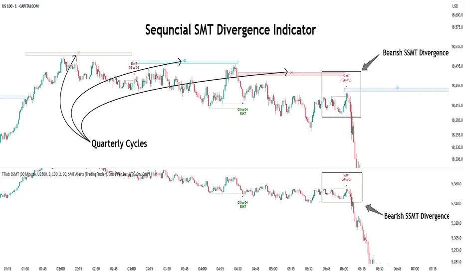
Fibonacci 3-D🟩 The Fibonacci 3-D indicator is a visual tool that introduces a three-dimensional approach to Fibonacci projections, leveraging market geometry. Unlike traditional Fibonacci tools that rely on two points and project horizontal levels, this indicator leverages slopes derived from three points to introduce a dynamic element into the calculations. The Fibonacci 3-D indicator uses three user-defined points to form a triangular structure, enabling multi-dimensional projections based on the relationships between the triangle’s sides.
This triangular framework forms the foundation for the indicator’s calculations, with each slope (⌳AB, ⌳AC, and ⌳BC) representing the rate of price change between its respective points. By incorporating these slopes into Fibonacci projections, the indicator provides an alternate approach to identifying potential support and resistance levels. The Fibonacci 3-D expands on traditional methods by integrating both historical price trends and recent momentum, offering deeper insights into market dynamics and aligning with broader market geometry.
The indicator operates across three modes, each defined by the triangular framework formed by three user-selected points (A, B, and C):
1-Dimensional (1-D): Fibonacci levels are based on a single side of the triangle, such as AB, AC, or BC. The slope of the selected side determines the angle of the projection, allowing users to analyze linear trends or directional price movements.
2-Dimensional (2-D): Combines two slopes derived from the sides of the triangle, such as AB and BC or AC and BC. This mode adds depth to the projections, accounting for both historical price swings and recent market momentum.
3-Dimensional (3-D): Integrates all three slopes into a unified projection. This mode captures the full geometric relationship between the points, revealing a comprehensive view of geometric market structure.
🌀 THEORY & CONCEPT 🌀
The Fibonacci 3-D indicator builds on the foundational principles of traditional Fibonacci analysis while expanding its scope to capture more intricate market structures. At its core, the indicator operates based on three user-selected points (A, B, and C), forming the vertices of a triangle that provides the structural basis for all calculations. This triangle determines the slopes, projections, and Fibonacci levels, aligning with the unique geometric relationships between the chosen points. By introducing multiple dimensions and leveraging this triangular framework, the indicator enables a deeper examination of price movements.
1️⃣ First Dimension (1-D)
In technical analysis, traditional Fibonacci retracement and extension tools operate as one-dimensional instruments. They rely on two price points, often a swing high and a swing low, to calculate and project horizontal levels at predefined Fibonacci ratios. These levels identify potential support and resistance zones based solely on the price difference between the selected points.
A one-dimensional Fibonacci showing levels derived from two price points (B and C).
The Fibonacci 3-D indicator extends this one-dimensional concept by introducing Ascending and Descending projection options. These options calculate the levels to align with the directional movement of price, creating sloped projections instead of purely horizontal levels.
1-D mode with an ascending projection along the ⌳BC slope aligned to the market's slope. Potential support is observed at 0.236 and 0.382, while resistance appears at 1.0 and 0.5.
2️⃣ Second Dimension (2-D)
The second dimension incorporates a second side of the triangle, introducing relationships between two slopes (e.g., ⌳AB and ⌳BC) to form a more dynamic three-point structure (A, B, and C) on the chart. This structure enables the indicator to move beyond the single-axis (price) calculations of traditional Fibonacci tools. The sides of the triangle (AB, AC, BC) represent slopes calculated as the rate of price change over time, capturing distinct components of market movement, such as trend direction and momentum.
2-D mode of the Fibonacci 3-D indicator using the ⌳AC slope with a descending projection. The Fibonacci projections align closely with observed market behavior, providing support at 0.236 and resistance at 0.618. Unlike traditional zigzag setups, this configuration uses two swing highs (A and B) and a swing low (C). The alignment along the descending slope highlights the geometric relationships between selected points in identifying potential support and resistance levels.
3️⃣ Third Dimension (3-D)
The third dimension expands the analysis by integrating all three slopes into a unified calculation, encompassing the entire triangle structure formed by points A, B, and C. Unlike the second dimension, which analyzes pairwise slope relationships, the 3-D mode reflects the combined geometry of the triangle. Each slope contributes a distinct perspective: AB and AC provide historical context, while BC emphasizes the most recent price movement and is given greater weight in the calculations to ensure projections remain responsive to current dynamics.
Using this integrated framework, the 3-D mode dynamically adjusts Fibonacci projections to balance long-term patterns and short-term momentum. The projections extend outward in alignment with the triangle’s geometry, offering a comprehensive framework for identifying potential support and resistance zones and capturing market structures beyond the scope of simpler 1-D or 2-D modes.
Three-dimensional Fibonacci projection using the ⌳AC slope, aligning closely with the market's directional movement. The projection highlights key levels: resistance at 0.0 and 0.618, and support at 1.0, 0.786, and 0.382.
By leveraging all three slopes simultaneously, the 3-D mode introduces a level of complexity particularly suited for volatile or non-linear markets. The weighted slope calculations ensure no single price movement dominates the analysis, allowing the projections to adapt dynamically to the broader market structure while remaining sensitive to recent momentum.
Three-dimensional ascending projection. In 3D mode, the indicator integrates all three slopes to calculate the angle of projection for the Fibonacci levels. The resulting projections adapt dynamically to the overall geometry of the ABC structure, aligning with the market’s current direction.
🔂 Interactions: Dimensions. Slope Source, Projections, and Orientation
The Dimensions , Projections , and Orientation settings work together to define Fibonacci projections within the triangular framework. Each setting plays a specific role in the geometric analysis of price movements.
♾️ Dimension determines which of the three modes (1-D, 2-D, or 3-D) is used for Fibonacci projections. In 1-D mode, the projections are based on a single side of the triangle, such as AB, AC, or BC. In 2-D mode, two sides are combined, producing levels based on their geometric relationship. The 3-D mode integrates all three sides of the triangle, calculating projections using weighted averages that emphasize the BC side for its relevance to recent price movement while maintaining historical context from the AB and AC sides.
A one-dimensional Fibonacci projection using the ⌳AB slope with a neutral projection. Important levels of interaction are highlighted: repeated resistance at Level 1.0 and repeated support at Levels 0.5 and 0.618. The projection aligns horizontally, reflecting the relationship between points A, B, and C while identifying recurring zones of market structure.
🧮 Slope Source determines which side of the triangle (AB, AC, or BC) serves as the foundation for Fibonacci projections. This selection directly impacts the calculations by specifying the slope that anchors the geometric relationships within the chosen Dimension mode (1-D, 2-D, or 3-D).
In 1-D mode, the selected Source defines the single side used for the projection. In 2-D and 3-D modes, the Source works in conjunction with other settings to refine projections by integrating the selected slope into the multi-dimensional framework.
One-dimensional Fibonacci projection using the ⌳AC Slope Source and Ascending projection. The projection continues on the AC slope line.
🎯 Projection controls the direction and alignment of Fibonacci levels. Neutral projections produce horizontal levels, similar to traditional Fibonacci tools. Ascending and Descending projections adjust the levels along the calculated slope to reflect market trends. These options allow the indicator’s outputs to align with different market behaviors.
An ascending projection along the ⌳BC slope aligns with resistance levels at 1.0, 0.618, and 0.236. The geometric relationship between points A, B, and C illustrates how the projection adapts to market structure, identifying resistance zones that may not be captured by traditional Fibonacci tools.
🧭 Orientation modifies the alignment of the setup area defined by points A, B, and C, which influences Fibonacci projections in 2-D and 3-D modes. In Default mode, the triangle aligns naturally based on the relative positions of points B and C. In Inverted mode, the geometric orientation of the setup area is reversed, altering the slope calculations while preserving the projection direction specified in the Projection setting. In 1-D mode, Orientation has no effect since only one side is used for the projection.
Adjusting the Orientation setting provides alternative views of how Fibonacci levels align with the market's structure. By recalibrating the triangle’s setup, the inverted orientation can highlight different relationships between the sides, providing additional perspectives on support and resistance zones.
2-D inverted. The ⌳AC slope defines the projection, and the inverted orientation adjusts the alignment of the setup area, altering the angles used in level calculations. Key levels are highlighted: resistance at 0.786, strong support at 0.5 and 0.236, and a resistance-turned-support interaction at 0.618.
🛠️ CONFIGURATION AND SETTINGS 🛠️
The Fibonacci 3-D indicator includes configurable settings to adjust its functionality and visual representation. These options include customization of the dimensions (1-D, 2-D, or 3-D), slope calculations, orientations, projections, Fibonacci levels, and visual elements.
When adding the indicator to a new chart, select three reference points (A, B, and C). These are usually set to recent swing points. All three points can be easily changed at any time by clicking on the reference point and dragging it to a new location.
By default, all settings are set to Auto . The indicator uses an internal algorithm to estimate the projections based on the orientation and relative positions of the reference points. However, all values can be overridden to reflect the user's interpretation of the current market geometry.
⚙️ Core Settings
Dimensions : Defines how many sides of the triangle formed by points A, B, and C are incorporated into the calculations for Fibonacci projections. This setting determines the level of complexity and detail in the analysis. 1-D : Projects levels along the angle of a single user-selected side of the triangle.
2-D : Projects levels based on a composite slope derived from the angles of two sides of the triangle.
3-D : Projects levels based on a composite slope derived from all three sides of the triangle (A-B, A-C, and B-C), providing a multi-dimensional projection that adapts to both historical and recent market movements.
Slope Source : Determines which side of the triangle is used as the basis for slope calculations. A–B: The slope between points A and B. In 1-D mode, this determines the projection. In 2-D and 3-D modes, it contributes to the composite slope calculation.
A–C: The slope between points A and C. In 1-D mode, this determines the projection. In 2-D and 3-D modes, it contributes to the composite slope calculation.
B--C: The slope between points B and C. In 1-D mode, this determines the projection. In 2-D and 3-D modes, it contributes to the composite slope calculation.
Orientation : Defines the triangle's orientation formed by points A, B, and C, influencing slope calculations. Auto : Automatically determines orientation based on the relative positions of points B and C. If point C is to the right of point B, the orientation is "normal." If point C is to the left, the orientation is inverted.
Inverted : Reverses the orientation set in "Auto" mode. This flips the triangle, reversing slope calculations ⌳AB becomes ⌳BA).
Projection : Determines the direction of Fibonacci projections: Auto : Automatically determines projection direction based on the triangle formed by A, B, and C.
Ascending : Projects the levels upward.
Neutral : Projects the levels horizontally, similar to traditional Fibonacci retracements.
Descending : Projects the levels downward.
⚙️ Fibonacci Level Settings Show or hide specific levels.
Level Value : Adjust Fibonacci ratios for each level. The 0.0 and 1.0 levels are fixed.
Color : Set level colors.
⚙️ Visibility Settings Show Setup : Toggle the display of the setup area, which includes the projected lines used in calculations.
Show Triangle : Toggle the display of the triangle formed by points A, B, and C.
Triangle Color : Set triangle line colors.
Show Point Labels : Toggle the display of labels for points A, B, and C.
Show Left/Right Labels : Toggle price labels on the left and right sides of the chart.
Fill % : Adjust the fill intensity between Fibonacci levels (0% for no fill, 100% for full fill).
Info : Set the location or hide the Slope Source and Dimension. If Orientation is Inverted , the Slope Source will display with an asterisk (*).
⚙️ Time-Price Points : Set the time and price for points A, B, and C, which define the Fibonacci projections.
A, B, and C Points : User-defined time and price coordinates that form the foundation of the indicator's calculations.
Interactive Adjustments : Changes made to points on the chart automatically synchronize with the settings panel and update projections in real time.
Notes
Unlike traditional Fibonacci tools that include extensions beyond 1.0 (e.g., 1.618 or 2.618), the Fibonacci 3-D indicator restricts Fibonacci levels to the range between 0.0 and 1.0. This is because the projections are tied directly to the proportional relationships along the sides of the triangle formed by points A, B, and C, rather than extending beyond its defined structure.
The indicator's calculations dynamically sort the user-defined A, B, and C points by time, ensuring point A is always the earliest, point C the latest, and point B the middle. This automatic sorting allows users to freely adjust the points directly on the chart without concern for their sequence, maintaining consistency in the triangular structure.
🖼️ ADDITIONAL CHART EXAMPLES 🖼️
Three-dimensional ⌳AC slope is used with an ascending projection, even as the broader market trend moves downward. Despite the apparent contradiction, the projected Fibonacci levels align closely with price action, identifying zones of support and resistance. These levels highlight smaller countertrend movements, such as pullbacks to 0.382 and 0.236, followed by continuations at resistance levels like 0.618 and 0.786.
In 2-D mode, an ascending projection based on the BC slope highlights the market's geometric structure. A setup triangle, defined by a swing high (A), a swing low (B), and another swing high (C), reveals Fibonacci projections aligning with support at 0.236, 0.382, and 0.5, and resistance at 0.618, 0.786, and 1.0, as shown by the green and red arrows. This demonstrates the ability to uncover dynamic support and resistance levels not calculated in traditional Fibonacci tools.
In 2-D mode with an ascending projection from the ⌳AB slope, price movement is contained within the 0.5 and 0.786 levels. The 0.5 level serves as support, while the 0.786 level acts as resistance, with price action consistently interacting with these boundaries.
An AC (2-D) ascending projection is derived from two swing highs (A and B) and a swing low (C), reflecting a non-linear market structure that deviates from traditional zigzag patterns. The ascending projection aligns closely with the market's upward trajectory, forming a channel between the 0.0 and 0.5 Fibonacci levels. Note how price action interacts with the projected levels, showing support at 0.236 and 0.382, with the 0.5 level acting as a mid-channel equilibrium.
Two-dimensional ascending Fibonacci projection using the ⌳AC slope. Arrows highlight resistance at 0.786 and support at 0.0 and 0.236. The projection follows the ⌳AC slope, reflecting the geometric relationship between points A, B, and C to identify these levels.
Three-dimensional Fibonacci projection using the ⌳AC slope, aligned with the actual market's directional trend. By removing additional Fibonacci levels, the image emphasizes key areas: resistance at Level 0.0 and support at Levels 1.0 and 0.5. The projection dynamically follows the ⌳AC slope, adapting to the market's structure as defined by points A, B, and C.
A three-dimensional configuration uses the ⌳AB slope as the baseline for projections while incorporating the geometric influence of point C. Only the 0.0 and 0.618 levels are enabled, emphasizing the relationship between support at 0.0 and resistance at 0.618. Unlike traditional Fibonacci tools, which operate in a single plane, this setup reveals levels that rely on the triangular relationship between points A, B, and C. The third dimension allows for projections that align more closely with the market’s structure and reflect its multi-dimensional geometry.
The Fibonacci 3-D indicator can adapt to non-traditional point selection. Point A serves as a swing low, while points B and C are swing highs, forming an unconventional configuration. ⌳The BC slope is used in 2-D mode with an inverted orientation, flipping the projection direction and revealing resistance at Level 0.786 and support at Levels 0.618 and 0.5.
⚠️ DISCLAIMER ⚠️
The Fibonacci 3-D indicator is a visual analysis tool designed to illustrate Fibonacci relationships. While the indicator employs precise mathematical and geometric formulas, no guarantee is made that its calculations will align with other Fibonacci tools or proprietary methods. Like all technical and visual indicators, the Fibonacci projections generated by this tool may appear to visually align with key price zones in hindsight. However, these projections are not intended as standalone signals for trading decisions. This indicator is intended for educational and analytical purposes, complementing other tools and methods of market analysis.
🧠 BEYOND THE CODE 🧠
The Fibonacci 3-D indicator, like other xxattaxx indicators , is designed to encourage both education and community engagement. Your feedback and insights are invaluable to refining and enhancing the Fibonacci 3-D indicator. We look forward to the creative applications, adaptations, and observations this tool inspires within the trading community.

Uptrick: Arbitrage OpportunityINTRODUCTION
This script, titled Uptrick: Arbitrage Monitor, is a Pine Script™ indicator that aims to help traders quickly visualize potential arbitrage scenarios across multiple cryptocurrency exchanges. Arbitrage, in general, involves taking advantage of price differences for the same asset across different trading platforms. By comparing market prices of the same symbol on two user-selected exchanges, as well as scanning a broader list of exchanges, this script attempts to signal areas where you might want to buy on one exchange and sell on another. It includes various graphical tools, calculations, and an optional Automated Detection signal feature, allowing users to incorporate more advanced data scanning into their trading decisions. Keep in mind that transaction fees must also be considered in real-world scenarios. These fees can negate potential profits and, in some cases, result in a net loss.
PURPOSE
The primary purpose of this indicator is to show potential percentage differences between the same cryptocurrency trading pairs on two different exchanges. This difference is displayed numerically, visually as a line chart, and it is also tested against user-defined thresholds. With the threshold in place, buy and sell signals can be generated. The script allows you to quickly gauge how significant a spread is between two exchanges and whether that spread surpasses a specified threshold. This is particularly useful for arbitrage trading, where an asset is bought at a lower price on one exchange and sold at a higher price on another, capitalizing on price discrepancies. By identifying these opportunities, traders can potentially secure profits across different markets.
WHY IT WAS MADE
This script was developed to help traders who frequently look for arbitrage opportunities in the fast-paced cryptocurrency market. Cryptocurrencies sometimes experience quick price divergences across different exchanges. By having an automated approach that compares and displays prices, traders can spend less time manually tracking price discrepancies and more time focusing on actual trading strategies. The script was also made with user customization in mind, allowing you to toggle an optional Automated-based approach and choose different moving average methods to smooth out the displayed price difference.
WHAT ARBITRAGE IS
Arbitrage is the practice of buying an asset on one market (or exchange) at a lower price and simultaneously selling it on another market where the price is higher, thus profiting from the price difference. In cryptocurrency markets, these price differentials can occur across multiple exchanges due to varying liquidity, trading volume, geographic factors, or market inefficiencies. Though sometimes small, these differences can be exploited for profit when approached methodically.
EXPLANATION OF INPUTS
The script includes a variety of user inputs that help tailor the indicator to your specific needs:
1. Compared Symbol 1: This is the primary symbol you want to track (for example, BTCUSDT). Make sure it's written in all capital and make sure that it's price from that exchange is available on Tradingview.
2. Compare Exchange 1: The first exchange on which the script will request pricing data for the chosen symbol.
3. Compared to Exchange: The second exchange, used for the comparison.
4. Opportunity Threshold (%): A percentage threshold that, when exceeded by the price difference, can trigger buy or sell signals.
5. Plot Style?: Allows you to choose between plotting the raw difference line or a moving average of that difference.
6. MA Type: Select among SMA, EMA, WMA, RMA, or HMA for your moving average calculation.
7. MA Length: The lookback period for the selected moving average.
8. Plot Buy/Sell Signals?: Enables or disables the plotting of arrows signaling potential buy or sell zones based on threshold crossovers.
9. Automated Detection?: Toggles an additional multi-exchange data scan feature that calculates the highest and lowest prices for the specified symbol across a predefined list of exchanges.
CALCULATIONS
At its core, the script calculates price1 and price2 using the request.security function to fetch close prices from two selected exchanges. The difference is measured as (price1 - price2) / price2 * 100. This results in a percentage that indicates how much higher or lower price1 is relative to price2. Additionally, the script calculates a slope for this difference, which helps color the line depending on whether it is trending up or down. If you choose the moving average option, the script will replace the raw difference data with one of several moving average calculations (SMA, EMA, WMA, RMA, or HMA).
The script also includes an iterative scan of up to 15 different exchanges for Automated detection, collecting the highest and lowest price across all those exchanges. If the Automated option is enabled, it compiles a potential recommendation: buy at the cheapest exchange price and sell at the most expensive one. The difference across all exchanges (allExDiffPercent) is calculated using (highestPriceAll - lowestPriceAll) / lowestPriceAll * 100.
WHAT AUTOMATED DETECTION SIGNAL DOES
If enabled, the Automated detection feature scans all 15 supported exchanges for the specified symbol. It then identifies the exchange with the highest price and the exchange with the lowest price. The script displays a recommended action: buy on the lowest-exchange price and sell on the highest-exchange price. While called “Automated,” it is essentially a multi-exchange data query that automates a portion of research by consolidating different price points. It does not replace thorough analysis or guaranteed execution; it simply provides an overview of potential extremes.
WHAT ALL-EX-DIFF IS
The variable allExDiffPercent is used to show the overall difference between the highest price and the lowest price found among the 15 pre-chosen exchanges. This figure can be useful for anyone wanting a big-picture view of how large the arbitrage spread might be across the broader market.
SIGNALS AND HOW THEY ARE GENERATED
The script provides two main modes of signal generation:
1. Raw Difference Mode: If the user chooses “Use Normal Line,” the script compares the percentage difference of the two selected exchanges (price1 and price2) to the user-defined threshold. When the difference crosses under the positive threshold, a sell signal is displayed (red arrow). Conversely, when the difference crosses above the negative threshold, a buy signal is displayed (green arrow).
2. Moving Average Mode: If the user selects “Use Moving Average,” the script instead references the moving average values (maValue). The signals fire under similar conditions but use the average line to gauge whether the threshold has been crossed.
HOW TO USE THE INDICATOR
1. Add the script to your chart in TradingView.
2. In the script’s settings panel, configure the symbol you wish to compare (for example, BTCUSDT), choose the two exchanges you want to evaluate, and set your desired threshold.
3. Optionally, pick a moving average type and length if you prefer a smoother representation of the difference.
4. Enable or disable buy/sell signals according to your preference.
5. If you’d like to see potential extremes among a broader list of exchanges, enable Automated Detection. Keep in mind that this feature runs additional security requests, so it might slow down performance on weaker devices or if you already have many scripts running.
EXCHANGES TO USE
The script currently supports up to 15 exchanges: BYBIT, BINANCE, MEXC, BLOFIN, BITGET, OKX, KUCOIN, COINBASE, COINEX, PHEMEX, POLONIEX, GATEIO, BITSTAMP, and KRAKEN. You can choose any two of these for direct comparison, and if you enable the Automated detection, it will attempt to query them all to find extremes in real time.
VISUALS
The exchanges and current prices & differences are all plotted in the table while the colored line represents the difference in the price. The two thresholds colored red are where signals are generated. A cross below the upper threshold is a sell signal and a cross above the lower threshold is a buy signal. In the line at the bottom, purple is a negative slope and aqua is a positive slope.
LIMITATIONS AND POTENTIAL PROBLEMS
If you enable too many visual elements such as signals, additional lines, and the Automated-based scanning table, you may find that your chart becomes cluttered, or text might overlap. One workaround is to remove and reapply the indicator to refresh its display. You may also want to reduce the number of displayed table rows by disabling some features if your chart becomes too crowded. Sometimes there might be an error that the price of an asset is not available on an exchange, to fix this, go and select another exchange to compare it to, or if it happens in Automated detection, choose a different asset, ideally more widely spread.
UNIQUENESS
This indicator stands out due to its multifaceted approach: it doesn’t just look at two exchanges but optionally scans up to 15 exchanges in real time, presenting users with a much broader view of the market. The dual-mode system (raw difference vs. moving average) allows for both immediate, unfiltered signals and smoother, noise-reduced signals depending on user preference. By default, it introduces dynamic visual cues through color changes when the slope of the difference transitions upward or downward. The optional Automated detection, while not a deep learning system, adds a functional intelligence layer by collating extreme price points from multiple exchanges in one place, thereby streamlining the manual research process. This combination of features gives the script a unique edge in the TradingView ecosystem, catering equally to novices wanting a straightforward approach and to advanced users looking for an aggregated multi-exchange analysis.
CONCLUSION
Uptrick: Arbitrage Monitor is a versatile and customizable Pine Script™ indicator that highlights price differences for a specified symbol between two user-selected exchanges. Through signals, threshold-based alerts, and optional Automated detection across multiple exchanges, it aims to support traders in identifying potential arbitrage opportunities quickly and efficiently. This script makes no guarantees of profitability but can serve as a valuable tool to add to your trading toolkit. Always use caution when implementing arbitrage strategies, and be mindful of market risks, exchange fees, and latency.
ADDITIONAL DISCLOSURES
This script is provided for educational and informational purposes only. It does not constitute financial advice or a guarantee of performance. Users are encouraged to conduct thorough research and consider the inherent risks of arbitrage trading. Market conditions can change rapidly, and orders may fail to execute at desired prices, especially when large price discrepancies attract competition from other traders.
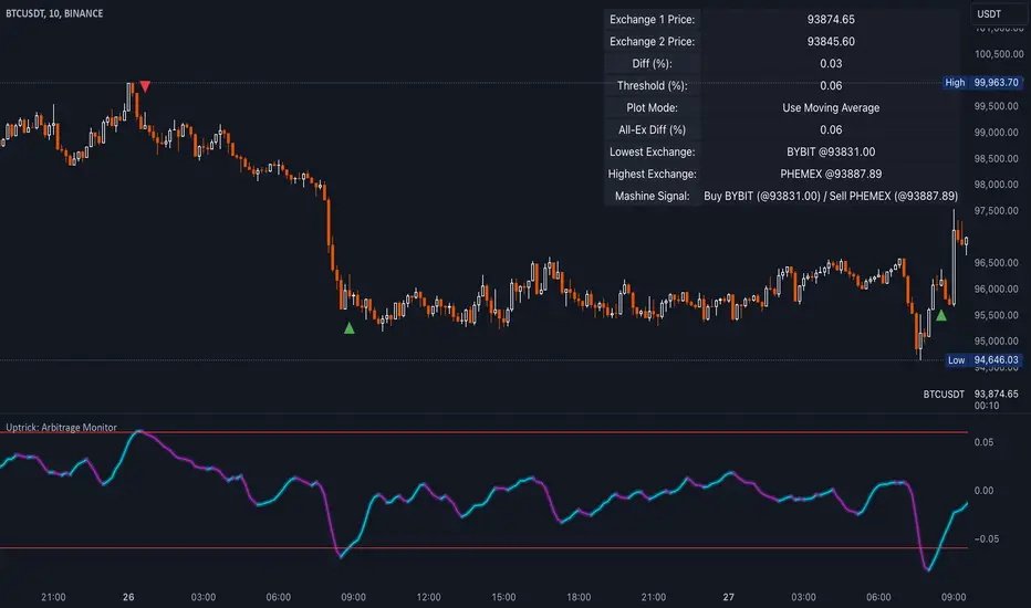
Advanced Pattern Detector**Script Overview**
**Indicator Name:** Advanced Pattern Detector
**Pine Script Version:** v5
**Indicator Type:** Overlaid on the chart (overlay=true)
**Main Features:**
- Detection and visualization of various technical patterns.
- Generation of BUY and SELL signals based on detected patterns.
- Display of Fibonacci levels to identify potential support and resistance levels.
- Ability to enable or disable each pattern through the indicator settings.
---
**Indicator Settings**
**Switches to Enable/Disable Patterns**
At the top of the indicator, there are parameters that allow the user to select which patterns will be displayed on the chart:
- Three Drives
- Rounding Top
- Rounding Bottom
- ZigZag Pattern
- Inverse Head and Shoulders
- Fibonacci Retracement
**Parameters for ZigZag**
Settings are also available for the ZigZag pattern, such as the depth of peak and trough detection, allowing the user to adjust the indicator's sensitivity to price changes.
---
**Pattern Detection**
Each pattern is implemented with its own logic, which checks specific conditions on the current bar (candle). Below are the main patterns:
1. **Three Drives**
- **Description:** This pattern consists of three consecutive price movements in one direction (up or down). It can signal the continuation of the current trend or its reversal.
- **How It Works:**
- **Upward Drive:** The indicator checks that the closing price of each subsequent candle is higher than the previous one for three bars.
- **Downward Drive:** The indicator checks that the closing price of each subsequent candle is lower than the previous one for three bars.
2. **Rounding Top**
- **Description:** A pattern representing a smooth decrease in maximum prices over several bars, which may indicate a potential downward trend reversal.
- **How It Works:**
- The indicator checks that the maximum prices of the last five bars are gradually decreasing, and the current bar shows a decrease in the maximum price.
3. **Rounding Bottom**
- **Description:** A pattern characterized by a smooth increase in minimum prices over several bars, signaling a possible upward trend reversal.
- **How It Works:**
- The indicator checks that the minimum prices of the last five bars are gradually increasing, and the current bar shows an increase in the minimum price.
4. **ZigZag Pattern**
- **Description:** Used to identify corrective movements on the chart. The pattern shows peak and trough points connected by lines, helping to visualize the main price movement.
- **How It Works:**
- The indicator uses a function to determine local maxima and minima based on the specified depth.
- Detected peaks and troughs are connected by lines to create a visual zigzag structure.
5. **Inverse Head and Shoulders**
- **Description:** An inverted head and shoulders formation signals a possible reversal of a downward trend to an upward one.
- **How It Works:**
- The indicator looks for three local minima: the left shoulder, the head (the lowest minimum), and the right shoulder.
- It checks that the left and right shoulders are approximately at the same level and below the head.
6. **Fibonacci Retracement Levels**
- **Description:** Automatically builds key Fibonacci levels based on the maximum and minimum prices over the last 50 bars. These levels are often used as potential support and resistance levels.
- **How It Works:**
- Daily, the minimum and maximum prices over the last 50 bars are calculated.
- Based on these values, Fibonacci levels are drawn: 100%, 23.6%, 38.2%, 50%, 61.8%, and 0%.
- Old levels are removed when a new day begins to keep the chart clean and up-to-date.
---
**Generation of Buy and Sell Signals**
The indicator combines the results of detected patterns to generate trading signals:
- **Buy Signals (BUY):**
- Rounding Bottom
- Three Drives Up
- Inverse Head and Shoulders
- ZigZag Low
- **Sell Signals (SELL):**
- Rounding Top
- Three Drives Down
- Inverse Head and Shoulders
- ZigZag High
**How It Works:**
- If one or more buy conditions are met, a "BUY" label is displayed below the corresponding bar on the chart.
- If one or more sell conditions are met, a "SELL" label is displayed above the corresponding bar on the chart.
---
**Visualization of Patterns on the Chart**
Each detected pattern is visualized using various graphical elements, allowing traders to easily identify them on the chart:
- **Three Drives Up:** Green upward triangle below the bar.
- **Three Drives Down:** Red downward triangle above the bar.
- **Rounding Top:** Orange "RT" label above the bar.
- **Rounding Bottom:** Blue "RB" label below the bar.
- **Inverse Head and Shoulders:** Turquoise "iH&S" label below the bar.
- **ZigZag High/Low:** Purple circles at the peaks and troughs of the zigzag.
---
**Displaying Fibonacci Levels**
Fibonacci levels are displayed as horizontal lines on the chart with corresponding labels. These levels help traders determine potential entry and exit points, as well as support and resistance levels.
---
**Drawing ZigZag Lines**
ZigZag lines connect the detected peaks and troughs, visualizing corrective movements. To avoid cluttering the chart, the number of lines is limited, and old lines are automatically removed as new ones are added.
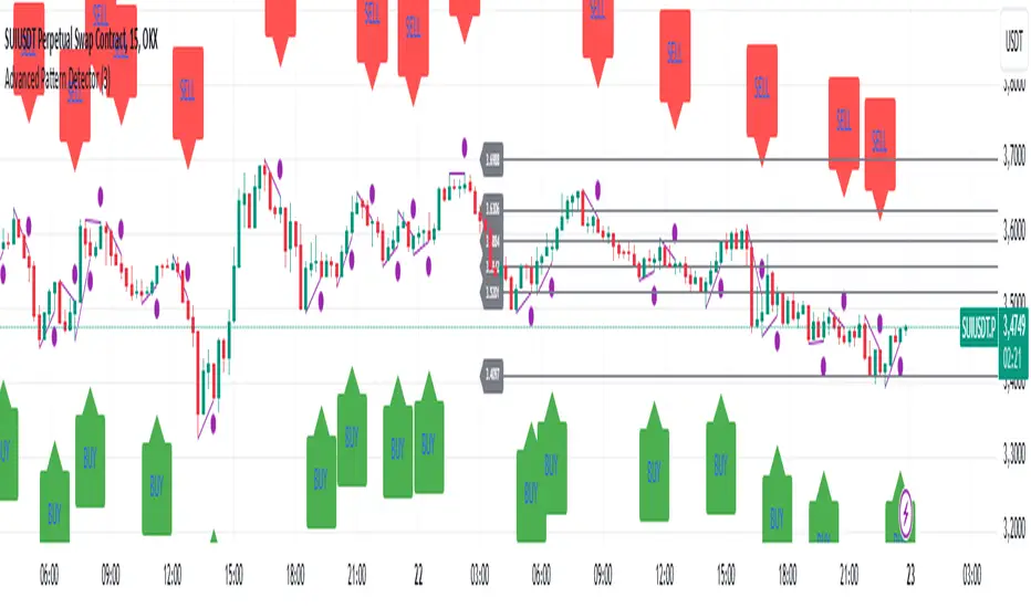
Supply and demandHi all!
This is my take on supply/demand. The gist is that it creates a zone if there is a big enough reaction. This is configurable in settings as "Minimum range (ATR factor)" (the Average True Length of length 14) that is the distance that the price must travel and "Reaction bars" that is the maximum number of bars that price must travel this distance. The zones that are shown are the ones that have a retest, break and retest or is unmitigated (untouched). If a zone is mitigated (entered) or broken it is temporarily hidden. For a zone to be created it needs to have this reaction and the previous bar does not.
So this script will show you zones that are fresh (unmitigated), retested or broken and retested. This means that the zones that are shown have "proven" that they are good zones through this. Basically it means that the script creates a bunch of zones and then picks the good once. This makes the script have some latency, but will hopefully give you good zones. A zone is completely removed if it's broken twice (it's okay if it's broken once and can still have a retest after it has flipped from previous supply (or resistance) into demand (or support)).
Here is a zone (the one that has the lowest opacity) that is broken and retested that could have resulted in a good long trade (the settings are default but has a stop in the beginning of 2024):
You have a setting to remove zones that are pierced (broken by price wicks). The following zone is pierced by price (in the beginning of May) that will not be shown after the start of May if you have "Pierced" checked (the indicator has default settings but a stop in the middle of April):
You have a trend section. Zones that create a reaction upwards can only be created if the trend is considered to be up, and vice versa. The options here are "SMA50" (the current price needs to be over the Simple Moving Average of length 50) and "SMA50, SMA200" (price needs to be over the Simple Moving Average of length 50 and the Simple Moving Average of length 50 needs to be over the Simple Moving Average of length 200). If these conditions are met the trend is considered to be up, otherwise it's down. You can disable this by choosing "No detection".
The zones that are shown also need to be within a limit (of the current price). This limit is 10 (factor of the Average True Range if length 14) by default. Set this to 0 to deactivate. This is useful for not showing zones that are far away from current price and therefore unlikely to be interacted with.
You can stop the calculation of zones (through the "Stop" value in the settings). This is useful to see if previous zones were any good. I used it in my testing of the script but left it because it can be nice to have.
The zones created by the script have different transparency based upon the zone's interaction. The clearest zones are the ones that are unmitigated, the second clearest ones are the ones having a retest and lastly the zones which are most unclear are the ones having a break and then a retest.
You can see the concept of this script to be a mix of supply/demand and support/resistance, having zones being unmitigated (untouched) as the most important but also show the zones having an interaction (in the form of a retest or a break and retest).
This is from a previous supply (or resistance) zone that has flipped into demand (or support) and has shown to be a good zone through a retest followed by a rally (default settings):
This zone has multiple retest and then rallies that could have given a good long trades (it has the default settings but a "Stop" time at 2022-01-14):
TODO:
- Create zones based on pivots
- Handle overlapping zones
- Incorporate volume in the creation and/or interaction with zones
- Add alerts
- Add ability to set maximum zone width
- Add ability to set the maximum number of retest bars
- ...?
The example for this publication has the default settings bit a "Stop" and a tighter "Limit" of 4.
I hope this explanation makes sense, let me know otherwise. Also let me know if you have any suggestions on improvements.
Best of trading luck!
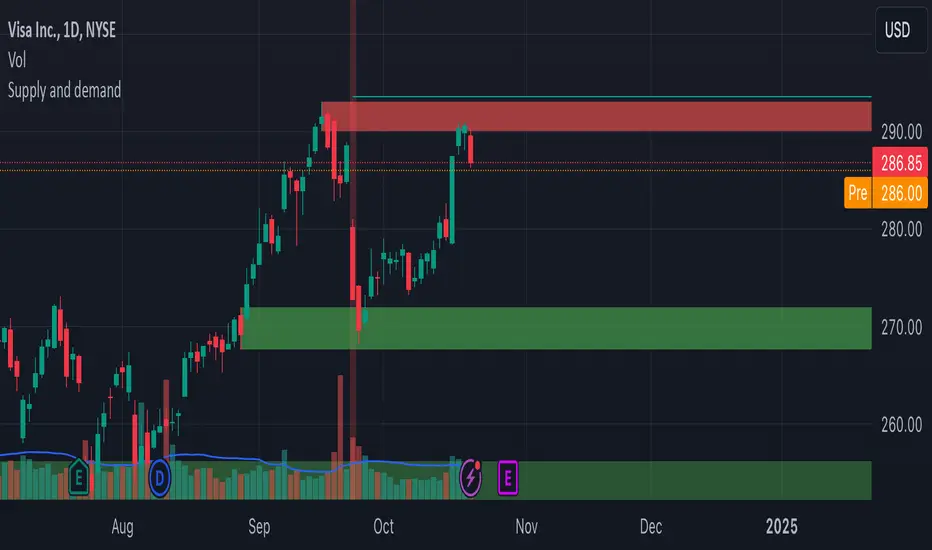
ICT Killzones and Sessions W/ Silver Bullet + MacrosForex and Equity Session Tracker with Killzones, Silver Bullet, and Macro Times
This Pine Script indicator is a comprehensive timekeeping tool designed specifically for ICT traders using any time-based strategy. It helps you visualize and keep track of forex and equity session times, kill zones, macro times, and silver bullet hours.
Features:
Session and Killzone Lines:
Green: London Open (LO)
White: New York (NY)
Orange: Australian (AU)
Purple: Asian (AS)
Includes AM and PM session markers.
Dotted/Striped Lines indicate overlapping kill zones within the session timeline.
Customization Options:
Display sessions and killzones in collapsed or full view.
Hide specific sessions or killzones based on your preferences.
Customize colors, texts, and sizes.
Option to hide drawings older than the current day.
Automatic Updates:
The indicator draws all lines and boxes at the start of a new day.
Automatically adjusts time-based boxes according to the New York timezone.
Killzone Time Windows (for indices):
London KZ: 02:00 - 05:00
New York AM KZ: 07:00 - 10:00
New York PM KZ: 13:30 - 16:00
Silver Bullet Times:
03:00 - 04:00
10:00 - 11:00
14:00 - 15:00
Macro Times:
02:33 - 03:00
04:03 - 04:30
08:50 - 09:10
09:50 - 10:10
10:50 - 11:10
11:50 - 12:50
Latest Update:
January 15:
Added option to automatically change text coloring based on the chart.
Included additional optional macro times per user request:
12:50 - 13:10
13:50 - 14:15
14:50 - 15:10
15:50 - 16:15
Usage:
To maximize your experience, minimize the pane where the script is drawn. This minimizes distractions while keeping the essential time markers visible. The script is designed to help traders by clearly annotating key trading periods without overwhelming their charts.
Originality and Justification:
This indicator uniquely integrates various time-based strategies essential for ICT traders. Unlike other indicators, it consolidates session times, kill zones, macro times, and silver bullet hours into one comprehensive tool. This allows traders to have a clear and organized view of critical trading periods, facilitating better decision-making.
Credits:
This script incorporates open-source elements with significant improvements to enhance functionality and user experience.
Forex and Equity Session Tracker with Killzones, Silver Bullet, and Macro Times
This Pine Script indicator is a comprehensive timekeeping tool designed specifically for ICT traders using any time-based strategy. It helps you visualize and keep track of forex and equity session times, kill zones, macro times, and silver bullet hours.
Features:
Session and Killzone Lines:
Green: London Open (LO)
White: New York (NY)
Orange: Australian (AU)
Purple: Asian (AS)
Includes AM and PM session markers.
Dotted/Striped Lines indicate overlapping kill zones within the session timeline.
Customization Options:
Display sessions and killzones in collapsed or full view.
Hide specific sessions or killzones based on your preferences.
Customize colors, texts, and sizes.
Option to hide drawings older than the current day.
Automatic Updates:
The indicator draws all lines and boxes at the start of a new day.
Automatically adjusts time-based boxes according to the New York timezone.
Killzone Time Windows (for indices):
London KZ: 02:00 - 05:00
New York AM KZ: 07:00 - 10:00
New York PM KZ: 13:30 - 16:00
Silver Bullet Times:
03:00 - 04:00
10:00 - 11:00
14:00 - 15:00
Macro Times:
02:33 - 03:00
04:03 - 04:30
08:50 - 09:10
09:50 - 10:10
10:50 - 11:10
11:50 - 12:50
Latest Update:
January 15:
Added option to automatically change text coloring based on the chart.
Included additional optional macro times per user request:
12:50 - 13:10
13:50 - 14:15
14:50 - 15:10
15:50 - 16:15
ICT Sessions and Kill Zones
What They Are:
ICT Sessions: These are specific times during the trading day when market activity is expected to be higher, such as the London Open, New York Open, and the Asian session.
Kill Zones: These are specific time windows within these sessions where the probability of significant price movements is higher. For example, the New York AM Kill Zone is typically from 8:30 AM to 11:00 AM EST.
How to Use Them:
Identify the Session: Determine which trading session you are in (London, New York, or Asian).
Focus on Kill Zones: Within that session, focus on the kill zones for potential trade setups. For instance, during the New York session, look for setups between 8:30 AM and 11:00 AM EST.
Silver Bullets
What They Are:
Silver Bullets: These are specific, high-probability trade setups that occur within the kill zones. They are designed to be "one shot, one kill" trades, meaning they aim for precise and effective entries and exits.
How to Use Them:
Time-Based Setup: Look for these setups within the designated kill zones. For example, between 10:00 AM and 11:00 AM for the New York AM session .
Chart Analysis: Start with higher time frames like the 15-minute chart and then refine down to 5-minute and 1-minute charts to identify imbalances or specific patterns .
Macros
What They Are:
Macros: These are broader market conditions and trends that influence your trading decisions. They include understanding the overall market direction, seasonal tendencies, and the Commitment of Traders (COT) reports.
How to Use Them:
Understand Market Conditions: Be aware of the macroeconomic factors and market conditions that could affect price movements.
Seasonal Tendencies: Know the seasonal patterns that might influence the market direction.
COT Reports: Use the Commitment of Traders reports to understand the positioning of large traders and commercial hedgers .
Putting It All Together
Preparation: Understand the macro conditions and review the COT reports.
Session and Kill Zone: Identify the trading session and focus on the kill zones.
Silver Bullet Setup: Look for high-probability setups within the kill zones using refined chart analysis.
Execution: Execute the trade with precision, aiming for a "one shot, one kill" outcome.
By following these steps, you can effectively use ICT sessions, kill zones, silver bullets, and macros to enhance your trading strategy.
Usage:
To maximize your experience, shrink the pane where the script is drawn. This minimizes distractions while keeping the essential time markers visible. The script is designed to help traders by clearly annotating key trading periods without overwhelming their charts.
Originality and Justification:
This indicator uniquely integrates various time-based strategies essential for ICT traders. Unlike other indicators, it consolidates session times, kill zones, macro times, and silver bullet hours into one comprehensive tool. This allows traders to have a clear and organized view of critical trading periods, facilitating better decision-making.
Credits:
This script incorporates open-source elements with significant improvements to enhance functionality and user experience. All credit goes to itradesize for the SB + Macro boxes
