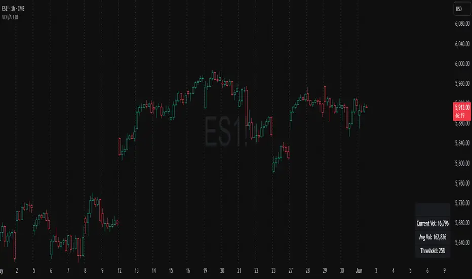
Volume Spike Alert & Overlay"Volume Spike Alert & Overlay" highlights unusually high trading volume on a chart. It calculates whether the current volume exceeds a user-defined percentage above the historical average and triggers an alert if it does. The information is also displayed in a customizable on-screen table.
What It Does
Monitors volume for each bar and compares it to an average over a user-defined lookback period.
Supports multiple smoothing methods (SMA, EMA, WMA, RMA) for calculating the average volume.
Triggers an alert when current volume exceeds the threshold percentage above the average.
Displays a table on the chart with:
Current Volume
Average Volume
Threshold Percentage
Optional empty row for spacing/formatting
How It Works
User Inputs:
lookbackPeriods: Number of bars used to calculate the average volume.
thresholdPercent: % above the average that triggers a volume spike alert.
smoothingType: Type of moving average used for volume calculation.
textColor, bgColor: Formatting for the display table.
tablePositionInput: Where the table appears on the chart (e.g., Bottom Right).
Toggles for showing/hiding parts of the table.
Volume Calculations:
Calculates current bar's volume.
Calculates average volume using the selected smoothing method.
Computes the threshold: avgVol * (1 + thresholdPercent / 100).
Compares current volume to threshold.
Table Display:
Dynamically creates a table with volume stats.
Adds rows based on user preferences.
Alerts:
alertcondition fires when currentVol crosses above the calculated threshold.
Message: "Volume Threshold Exceeded"
Usage Examples
Example 1: Spotting High Activity
Apply the script to a stock like AAPL on a 5-minute chart.
Set lookbackPeriods to 20 and thresholdPercent to 30.
Use EMA for more reactive volume tracking.
When volume spikes more than 30% above the 20-period EMA, an alert triggers.
Example 2: Day Trading Filter
For scalpers, apply it to a 1-minute crypto chart (e.g., BTC/USDT).
Set thresholdPercent to 50 to catch only strong surges.
Position the table at the top left and reduce visible info for a clean layout.
Example 3: Long-Term Context
On a daily chart, use SMA and set lookbackPeriods to 50.
Helps identify breakout moves supported by strong volume.
How this is different from Trading View's Volume indicator:
The standard volume plot from trading view allows users to set a alert when the average line is crossed, but it does not allow you to set a custom percentage at which to trigger an alert. This indicator will allow you to set any percentage you wish to monitor and above that percentage threshold will trigger your alert.
===== ORIGINAL DESCRIPTION =====
Volume Spike Alert & Overlay
This indicator will display the following as an overlay on your chart:
Current volume
Average Volume
Threshold for Alert
Description:
This indicator will display the current bar volume based on the chart time frame,
display the average volume based on selected conditions,
allow user selectable threshold over the average volume to trigger an alert.
Options:
Average lookback period
Smoothing type
Alert Threshold %
Enable / Disable Each Value
Change Text Color
Change Background Color
Change Table location
Add/Remove extra row for placement in top corner
Usage Example:
I use this indicator to alert when the current volume exceeds the average volume by a specified percentage to alert to volume spikes.
Set the threshold to 25% in the settings
Create an alert by clicking on the 3 dots on the right of the indicator title on the chart
When the threshold is exceeded the alert will trigger
חפש סקריפטים עבור "text"
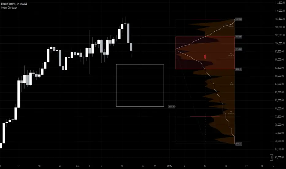
Intrabar DistributionThe Intrabar Distribution publication is an extension of the Intrabar BoxPlot publication. Besides a boxplot, it showcases price and volume distribution using intrabar Lower Timeframe (LTF) values (close) which can be displayed on the chart or in a separate pane.
🔶 USAGE
Intrabar Distribution has several features, users can display:
Recent candle for comparison against the other features
Boxplot of recent candle
Price distribution (optionally displayed as a curve)
Volume distribution
🔹 Recent candle / Boxplot
The middle 50% intrabar close values (Interquartile range, or IQR) are shown as a box, where the upper limit is percentile 75 (p75), and the lower limit is percentile 25 (p25). The dashed lines show the addition/subtraction of 1.5*IQR. All values out of range are considered outliers. They are displayed as white dots within the IQR*1.5 range or white X's when beyond the IQR*3 range (extreme outliers).
By showing the middle 50% intrabar values through a box, we can more easily see where the intrabar activity is mainly situated.
Note in the example above an upward-directed candle with a negative volume delta, displayed as a red box and dot (see further).
As seen in the following example, compared against the recent candle (grey candle at the left), most of the intrabar activity lies just beneath the opening price.
Note that results will be more accurate when more data is available, which can be done by making the difference between the current timeframe and the intrabar timeframe large enough.
🔹 Price / Volume distribution
The price and volume distribution can be helpful for highlighting areas of interest.
Here, we can see two areas where intrabar closing prices are mainly positioned.
The following example shows three successive bars. The recent bar is displayed on the left side, together with the volume distribution. The boxplot and price distribution are displayed on the right.
You can see the difference between volume and price distribution.
At the first bar, most price activity is at the top, while most of the volume was generated at the bottom; in other words, the price got briefly in the bottom region, with high volume before it returned.
At the second bar, price and volume are relatively equally distributed, which fits for indecisiveness.
The third bar shows more volume at a higher region; most intrabar closing prices are above the closing price.
Following example shows the same with 'Curve shaped' enabled (Settings: 'Price Distribution')
When 'Curve shaped' is enabled, lines/labels are shown with the standard deviation distance.
A blue 'guide line' can be enabled for easier interpretation.
🔹 Volume Delta
When there is a discrepancy between the delta volume and direction of the candle, this will be displayed as follows:
Red candle: when the sum of the volume of green intrabars is higher than the sum of the volume of red intrabars, the 'mean dot' will be coloured green.
Green candle: when the sum of the volume of red intrabars is higher than the sum of the volume of green intrabars, the 'mean dot' will be coloured red.
🔶 DETAILS
The intrabar values are sorted and split in parts/sections. The number of values in each section is displayed as a white line
The same principle applies to volume distribution, where the sum of volume per section is displayed as an orange area.
The boxplot displays several price values
Last close price
Highest / lowest intrabar close price
Median
p25 / p75
🔹 LTF settings
When 'Auto' is enabled (Settings, LTF), the LTF will be the nearest possible x times smaller TF than the current TF. When 'Premium' is disabled, the minimum TF will always be 1 minute to ensure TradingView plans lower than Premium don't get an error.
Examples with current Daily TF (when Premium is enabled):
500 : 3 minute LTF
1500 (default): 1 minute LTF
5000: 30 seconds LTF (1 minute if Premium is disabled)
🔶 SETTINGS
Location: Chart / Pane (when pane is opted, move the indicator to a separate pane as well)
Parts: divides the intrabar close values into parts/sections
Offset: offsets every drawing at once
Width: width of drawings, only applicable on "location: chart"
Label size: size of price labels
🔹 LTF
LTF: LTF setting
Auto + multiple: Adjusts the initial set LTF
Premium: Enable when your TradingView plan is Premium or higher
🔹 Current Bar
Display toggle + color setting
Offset: offsets only the 'Current Bar' drawing
🔹 Intrabar Boxplot
Display toggle + Colors, dependable on different circumstances.
Up: Price goes up, with more bullish than bearish intrabar volume.
Up-: Price goes up, with more bearish than bullish intrabar volume.
Down: Price goes down, with more bearish than bullish intrabar volume.
Down+: Price goes down, with more bullish than bearish intrabar volume.
Offset: offsets only the 'Boxplot' drawing
🔹 Price distribution
Display toggle + Color.
Curve Shaped
Guide Lines: Display 2 blue lines
Display Price: Show price of 'x' standard deviation
Offset: offsets only the 'Price distribution' drawing
Label size: size of price labels (standard deviation)
🔹 Volume distribution
Display toggle + Color.
Offset: offsets only the 'Volume distribution' drawing
🔹 Table
Show TF: Show intrabar Timeframe.
Textcolor
Size Table: Text Size
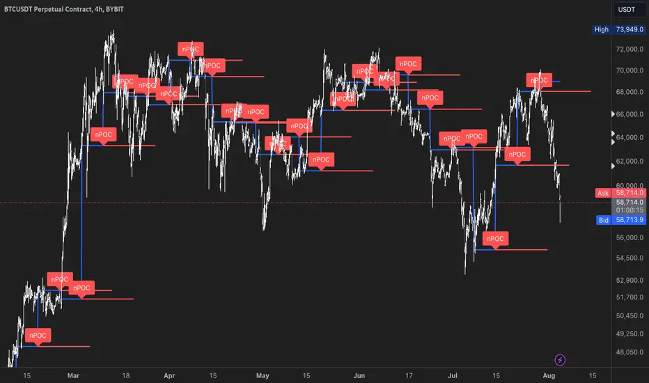
nPOC Levels by Tyler### Explanation of the Pine Script
This Pine Script identifies and displays weekly naked Points of Control (nPOCs) on a TradingView chart. An nPOC represents a Point of Control (POC) from a previous week that has not been revisited by price action in subsequent weeks. These nPOCs are extended to the right as horizontal lines, indicating potential support or resistance levels.
#### Script Overview
1. **Indicator Declaration:**
```pinescript
//@version=5
indicator("Weekly nPOCs", overlay=true)
```
- The script is defined as a version 5 Pine Script.
- The `indicator` function sets the script's name ("Weekly nPOCs") and specifies that the indicator should be overlaid on the price chart (`overlay=true`).
2. **Function to Calculate POC:**
```pinescript
f_poc(_hl2, _vol) =>
var float vol_profile = na
if (na(vol_profile))
vol_profile := array.new_float(100, 0.0)
_bin_size = (high - low) / 100
for i = 0 to 99
if _hl2 >= low + i * _bin_size and _hl2 < low + (i + 1) * _bin_size
array.set(vol_profile, i, array.get(vol_profile, i) + _vol)
max_volume = array.max(vol_profile)
poc_index = array.indexof(vol_profile, max_volume)
poc_price = low + poc_index * _bin_size + _bin_size / 2
poc_price
```
- The function `f_poc` calculates the Point of Control (POC) for a given period.
- It takes two parameters: `_hl2` (the average of the high and low prices) and `_vol` (volume).
- A volume profile array (`vol_profile`) is initialized to store volume data across different price bins.
- The price range between the high and low is divided into 100 bins (`_bin_size`).
- The function iterates over each bin, accumulating the volumes for prices within each bin.
- The bin with the maximum volume is identified as the POC (`poc_price`).
3. **Variables to Store Weekly Data:**
```pinescript
var float poc = na
var float prev_poc = na
var line poc_lines = na
if na(poc_lines)
poc_lines := array.new_line(0)
```
- `poc` stores the current week's POC.
- `prev_poc` stores the previous week's POC.
- `poc_lines` is an array to store lines representing nPOCs. The array is initialized if it is `na` (not initialized).
4. **Calculate Weekly POC:**
```pinescript
is_new_week = ta.change(time('W')) != 0
if (is_new_week)
prev_poc := poc
poc := f_poc(hl2, volume)
if not na(prev_poc)
line new_poc_line = line.new(x1=bar_index, y1=prev_poc, x2=bar_index + 100, y2=prev_poc, color=color.red, width=2)
label.new(x=bar_index, y=prev_poc, text="nPOC", style=label.style_label_down, color=color.red, textcolor=color.white)
array.push(poc_lines, new_poc_line)
```
- `is_new_week` checks if the current bar is the start of a new week using the `ta.change(time('W'))` function.
- If it's a new week, the previous week's POC is stored in `prev_poc`, and the current week's POC is calculated using `f_poc`.
- If `prev_poc` is not `na`, a new line (`new_poc_line`) representing the nPOC is created, extending it to the right (for 100 bars).
- A label is created at the `prev_poc` level, marking it as "nPOC".
- The new line is added to the `poc_lines` array.
5. **Remove Old Lines:**
```pinescript
if array.size(poc_lines) > 52
line.delete(array.shift(poc_lines))
```
- This section ensures that only the last 52 weeks of nPOCs are kept to avoid cluttering the chart.
- If the `poc_lines` array contains more than 52 lines, the oldest line is deleted using `array.shift`.
6. **Plot the Current Week's POC as a Reference:**
```pinescript
plot(poc, title="Current Weekly POC", color=color.blue, linewidth=2, style=plot.style_line)
```
- The current week's POC is plotted as a blue line on the chart for reference.
#### Summary
This script calculates and identifies weekly Points of Control (POCs) and marks them as nPOCs if they remain untouched by subsequent price action. These nPOCs are displayed as horizontal lines extending to the right, providing traders with potential support or resistance levels. The script also manages the number of lines plotted to maintain a clear and uncluttered chart.
itradesize /\ Silver Bullet x Macro x KillzoneThis indicator shows the best way to annotate ICT Killzones, Silver Bullet and Macro times on the chart. With the help of a new pane, it will not distract your chart and will not cause any distractions to your eye, or brain but you can see when will they happen.
The indicator also draws everything beforehand when a proper new day starts.
You can customize them how you want to show up.
Collapsed or full view?
You can hide any of them and keep only the ones you would like to.
All the colors can be customized, texts & sizes or just use shortened texts and you are also able to hide those drawings which are older than the actual day.
You should minimize the pane where the script has been automatically drawn to therefore you will have the best experience and not show any distractions.
The script automatically shows the time-based boxes, based on the New York timezone.
Killzone Time windows ( for indices ):
London KZ 02:00 - 05:00
New York AM KZ 07:00 - 10:00
New York PM KZ 13:30 - 16:00
Silver Bullet times:
03:00 - 04:00
10:00 - 11:00
14:00 - 15:00
Macro times:
02:33 - 03:00
04:03 - 04:30
08:50 - 0910
09:50 - 10:10
10:50 - 11:10
11:50 - 12:50

ZigzagLiteLibrary "ZigzagLite"
Lighter version of the Zigzag Library. Without indicators and sub-component divisions
method getPrices(pivots)
Gets the array of prices from array of Pivots
Namespace types: Pivot
Parameters:
pivots (Pivot ) : array array of Pivot objects
Returns: array array of pivot prices
method getBars(pivots)
Gets the array of bars from array of Pivots
Namespace types: Pivot
Parameters:
pivots (Pivot ) : array array of Pivot objects
Returns: array array of pivot bar indices
method getPoints(pivots)
Gets the array of chart.point from array of Pivots
Namespace types: Pivot
Parameters:
pivots (Pivot ) : array array of Pivot objects
Returns: array array of pivot points
method getPoints(this)
Namespace types: Zigzag
Parameters:
this (Zigzag)
method calculate(this, ohlc, ltfHighTime, ltfLowTime)
Calculate zigzag based on input values and indicator values
Namespace types: Zigzag
Parameters:
this (Zigzag) : Zigzag object
ohlc (float ) : Array containing OHLC values. Can also have custom values for which zigzag to be calculated
ltfHighTime (int) : Used for multi timeframe zigzags when called within request.security. Default value is current timeframe open time.
ltfLowTime (int) : Used for multi timeframe zigzags when called within request.security. Default value is current timeframe open time.
Returns: current Zigzag object
method calculate(this)
Calculate zigzag based on properties embedded within Zigzag object
Namespace types: Zigzag
Parameters:
this (Zigzag) : Zigzag object
Returns: current Zigzag object
method nextlevel(this)
Namespace types: Zigzag
Parameters:
this (Zigzag)
method clear(this)
Clears zigzag drawings array
Namespace types: ZigzagDrawing
Parameters:
this (ZigzagDrawing ) : array
Returns: void
method clear(this)
Clears zigzag drawings array
Namespace types: ZigzagDrawingPL
Parameters:
this (ZigzagDrawingPL ) : array
Returns: void
method drawplain(this)
draws fresh zigzag based on properties embedded in ZigzagDrawing object without trying to calculate
Namespace types: ZigzagDrawing
Parameters:
this (ZigzagDrawing) : ZigzagDrawing object
Returns: ZigzagDrawing object
method drawplain(this)
draws fresh zigzag based on properties embedded in ZigzagDrawingPL object without trying to calculate
Namespace types: ZigzagDrawingPL
Parameters:
this (ZigzagDrawingPL) : ZigzagDrawingPL object
Returns: ZigzagDrawingPL object
method drawfresh(this, ohlc)
draws fresh zigzag based on properties embedded in ZigzagDrawing object
Namespace types: ZigzagDrawing
Parameters:
this (ZigzagDrawing) : ZigzagDrawing object
ohlc (float ) : values on which the zigzag needs to be calculated and drawn. If not set will use regular OHLC
Returns: ZigzagDrawing object
method drawcontinuous(this, ohlc)
draws zigzag based on the zigzagmatrix input
Namespace types: ZigzagDrawing
Parameters:
this (ZigzagDrawing) : ZigzagDrawing object
ohlc (float ) : values on which the zigzag needs to be calculated and drawn. If not set will use regular OHLC
Returns:
PivotCandle
PivotCandle represents data of the candle which forms either pivot High or pivot low or both
Fields:
_high (series float) : High price of candle forming the pivot
_low (series float) : Low price of candle forming the pivot
length (series int) : Pivot length
pHighBar (series int) : represents number of bar back the pivot High occurred.
pLowBar (series int) : represents number of bar back the pivot Low occurred.
pHigh (series float) : Pivot High Price
pLow (series float) : Pivot Low Price
Pivot
Pivot refers to zigzag pivot. Each pivot can contain various data
Fields:
point (chart.point) : pivot point coordinates
dir (series int) : direction of the pivot. Valid values are 1, -1, 2, -2
level (series int) : is used for multi level zigzags. For single level, it will always be 0
ratio (series float) : Price Ratio based on previous two pivots
sizeRatio (series float)
ZigzagFlags
Flags required for drawing zigzag. Only used internally in zigzag calculation. Should not set the values explicitly
Fields:
newPivot (series bool) : true if the calculation resulted in new pivot
doublePivot (series bool) : true if the calculation resulted in two pivots on same bar
updateLastPivot (series bool) : true if new pivot calculated replaces the old one.
Zigzag
Zigzag object which contains whole zigzag calculation parameters and pivots
Fields:
length (series int) : Zigzag length. Default value is 5
numberOfPivots (series int) : max number of pivots to hold in the calculation. Default value is 20
offset (series int) : Bar offset to be considered for calculation of zigzag. Default is 0 - which means calculation is done based on the latest bar.
level (series int) : Zigzag calculation level - used in multi level recursive zigzags
zigzagPivots (Pivot ) : array which holds the last n pivots calculated.
flags (ZigzagFlags) : ZigzagFlags object which is required for continuous drawing of zigzag lines.
ZigzagObject
Zigzag Drawing Object
Fields:
zigzagLine (series line) : Line joining two pivots
zigzagLabel (series label) : Label which can be used for drawing the values, ratios, directions etc.
ZigzagProperties
Object which holds properties of zigzag drawing. To be used along with ZigzagDrawing
Fields:
lineColor (series color) : Zigzag line color. Default is color.blue
lineWidth (series int) : Zigzag line width. Default is 1
lineStyle (series string) : Zigzag line style. Default is line.style_solid.
showLabel (series bool) : If set, the drawing will show labels on each pivot. Default is false
textColor (series color) : Text color of the labels. Only applicable if showLabel is set to true.
maxObjects (series int) : Max number of zigzag lines to display. Default is 300
xloc (series string) : Time/Bar reference to be used for zigzag drawing. Default is Time - xloc.bar_time.
curved (series bool) : Boolean field to print curved zigzag - used only with polyline implementation
ZigzagDrawing
Object which holds complete zigzag drawing objects and properties.
Fields:
zigzag (Zigzag) : Zigzag object which holds the calculations.
properties (ZigzagProperties) : ZigzagProperties object which is used for setting the display styles of zigzag
drawings (ZigzagObject ) : array which contains lines and labels of zigzag drawing.
ZigzagDrawingPL
Object which holds complete zigzag drawing objects and properties - polyline version
Fields:
zigzag (Zigzag) : Zigzag object which holds the calculations.
properties (ZigzagProperties) : ZigzagProperties object which is used for setting the display styles of zigzag
zigzagLabels (label )
zigzagLine (series polyline) : polyline object of zigzag lines

ZigzagLibrary "Zigzag"
Zigzag related user defined types. Depends on DrawingTypes library for basic types
method tostring(this, sortKeys, sortOrder, includeKeys)
Converts ZigzagTypes/Pivot object to string representation
Namespace types: Pivot
Parameters:
this (Pivot) : ZigzagTypes/Pivot
sortKeys (bool) : If set to true, string output is sorted by keys.
sortOrder (int) : Applicable only if sortKeys is set to true. Positive number will sort them in ascending order whreas negative numer will sort them in descending order. Passing 0 will not sort the keys
includeKeys (string ) : Array of string containing selective keys. Optional parmaeter. If not provided, all the keys are considered
Returns: string representation of ZigzagTypes/Pivot
method tostring(this, sortKeys, sortOrder, includeKeys)
Converts Array of Pivot objects to string representation
Namespace types: Pivot
Parameters:
this (Pivot ) : Pivot object array
sortKeys (bool) : If set to true, string output is sorted by keys.
sortOrder (int) : Applicable only if sortKeys is set to true. Positive number will sort them in ascending order whreas negative numer will sort them in descending order. Passing 0 will not sort the keys
includeKeys (string ) : Array of string containing selective keys. Optional parmaeter. If not provided, all the keys are considered
Returns: string representation of Pivot object array
method tostring(this)
Converts ZigzagFlags object to string representation
Namespace types: ZigzagFlags
Parameters:
this (ZigzagFlags) : ZigzagFlags object
Returns: string representation of ZigzagFlags
method tostring(this, sortKeys, sortOrder, includeKeys)
Converts ZigzagTypes/Zigzag object to string representation
Namespace types: Zigzag
Parameters:
this (Zigzag) : ZigzagTypes/Zigzagobject
sortKeys (bool) : If set to true, string output is sorted by keys.
sortOrder (int) : Applicable only if sortKeys is set to true. Positive number will sort them in ascending order whreas negative numer will sort them in descending order. Passing 0 will not sort the keys
includeKeys (string ) : Array of string containing selective keys. Optional parmaeter. If not provided, all the keys are considered
Returns: string representation of ZigzagTypes/Zigzag
method calculate(this, ohlc, indicators, indicatorNames)
Calculate zigzag based on input values and indicator values
Namespace types: Zigzag
Parameters:
this (Zigzag) : Zigzag object
ohlc (float ) : Array containing OHLC values. Can also have custom values for which zigzag to be calculated
indicators (matrix) : Array of indicator values
indicatorNames (string ) : Array of indicator names for which values are present. Size of indicators array should be equal to that of indicatorNames
Returns: current Zigzag object
method calculate(this)
Calculate zigzag based on properties embedded within Zigzag object
Namespace types: Zigzag
Parameters:
this (Zigzag) : Zigzag object
Returns: current Zigzag object
method nextlevel(this)
Calculate Next Level Zigzag based on the current calculated zigzag object
Namespace types: Zigzag
Parameters:
this (Zigzag) : Zigzag object
Returns: Next Level Zigzag object
method clear(this)
Clears zigzag drawings array
Namespace types: ZigzagDrawing
Parameters:
this (ZigzagDrawing ) : array
Returns: void
method drawplain(this)
draws fresh zigzag based on properties embedded in ZigzagDrawing object without trying to calculate
Namespace types: ZigzagDrawing
Parameters:
this (ZigzagDrawing) : ZigzagDrawing object
Returns: ZigzagDrawing object
method drawfresh(this, ohlc, indicators, indicatorNames)
draws fresh zigzag based on properties embedded in ZigzagDrawing object
Namespace types: ZigzagDrawing
Parameters:
this (ZigzagDrawing) : ZigzagDrawing object
ohlc (float ) : values on which the zigzag needs to be calculated and drawn. If not set will use regular OHLC
indicators (matrix) : Array of indicator values
indicatorNames (string ) : Array of indicator names for which values are present. Size of indicators array should be equal to that of indicatorNames
Returns: ZigzagDrawing object
method drawcontinuous(this, ohlc, indicators, indicatorNames)
draws zigzag based on the zigzagmatrix input
Namespace types: ZigzagDrawing
Parameters:
this (ZigzagDrawing) : ZigzagDrawing object
ohlc (float ) : values on which the zigzag needs to be calculated and drawn. If not set will use regular OHLC
indicators (matrix) : Array of indicator values
indicatorNames (string ) : Array of indicator names for which values are present. Size of indicators array should be equal to that of indicatorNames
Returns:
method getPrices(pivots)
Namespace types: Pivot
Parameters:
pivots (Pivot )
method getBars(pivots)
Namespace types: Pivot
Parameters:
pivots (Pivot )
Indicator
Indicator is collection of indicator values applied on high, low and close
Fields:
indicatorHigh (series float) : Indicator Value applied on High
indicatorLow (series float) : Indicator Value applied on Low
PivotCandle
PivotCandle represents data of the candle which forms either pivot High or pivot low or both
Fields:
_high (series float) : High price of candle forming the pivot
_low (series float) : Low price of candle forming the pivot
length (series int) : Pivot length
pHighBar (series int) : represents number of bar back the pivot High occurred.
pLowBar (series int) : represents number of bar back the pivot Low occurred.
pHigh (series float) : Pivot High Price
pLow (series float) : Pivot Low Price
indicators (Indicator ) : Array of Indicators - allows to add multiple
Pivot
Pivot refers to zigzag pivot. Each pivot can contain various data
Fields:
point (chart.point) : pivot point coordinates
dir (series int) : direction of the pivot. Valid values are 1, -1, 2, -2
level (series int) : is used for multi level zigzags. For single level, it will always be 0
componentIndex (series int) : is the lower level zigzag array index for given pivot. Used only in multi level Zigzag Pivots
subComponents (series int) : is the number of sub waves per each zigzag wave. Only applicable for multi level zigzags
microComponents (series int) : is the number of base zigzag components in a zigzag wave
ratio (series float) : Price Ratio based on previous two pivots
sizeRatio (series float)
subPivots (Pivot )
indicatorNames (string ) : Names of the indicators applied on zigzag
indicatorValues (float ) : Values of the indicators applied on zigzag
indicatorRatios (float ) : Ratios of the indicators applied on zigzag based on previous 2 pivots
ZigzagFlags
Flags required for drawing zigzag. Only used internally in zigzag calculation. Should not set the values explicitly
Fields:
newPivot (series bool) : true if the calculation resulted in new pivot
doublePivot (series bool) : true if the calculation resulted in two pivots on same bar
updateLastPivot (series bool) : true if new pivot calculated replaces the old one.
Zigzag
Zigzag object which contains whole zigzag calculation parameters and pivots
Fields:
length (series int) : Zigzag length. Default value is 5
numberOfPivots (series int) : max number of pivots to hold in the calculation. Default value is 20
offset (series int) : Bar offset to be considered for calculation of zigzag. Default is 0 - which means calculation is done based on the latest bar.
level (series int) : Zigzag calculation level - used in multi level recursive zigzags
zigzagPivots (Pivot ) : array which holds the last n pivots calculated.
flags (ZigzagFlags) : ZigzagFlags object which is required for continuous drawing of zigzag lines.
ZigzagObject
Zigzag Drawing Object
Fields:
zigzagLine (series line) : Line joining two pivots
zigzagLabel (series label) : Label which can be used for drawing the values, ratios, directions etc.
ZigzagProperties
Object which holds properties of zigzag drawing. To be used along with ZigzagDrawing
Fields:
lineColor (series color) : Zigzag line color. Default is color.blue
lineWidth (series int) : Zigzag line width. Default is 1
lineStyle (series string) : Zigzag line style. Default is line.style_solid.
showLabel (series bool) : If set, the drawing will show labels on each pivot. Default is false
textColor (series color) : Text color of the labels. Only applicable if showLabel is set to true.
maxObjects (series int) : Max number of zigzag lines to display. Default is 300
xloc (series string) : Time/Bar reference to be used for zigzag drawing. Default is Time - xloc.bar_time.
ZigzagDrawing
Object which holds complete zigzag drawing objects and properties.
Fields:
zigzag (Zigzag) : Zigzag object which holds the calculations.
properties (ZigzagProperties) : ZigzagProperties object which is used for setting the display styles of zigzag
drawings (ZigzagObject ) : array which contains lines and labels of zigzag drawing.

ZigzagTypesLibrary "ZigzagTypes"
Zigzag related user defined types. Depends on DrawingTypes library for basic types
Indicator
Indicator is collection of indicator values applied on high, low and close
Fields:
indicatorHigh : Indicator Value applied on High
indicatorLow : Indicator Value applied on Low
PivotCandle
PivotCandle represents data of the candle which forms either pivot High or pivot low or both
Fields:
_high : High price of candle forming the pivot
_low : Low price of candle forming the pivot
length : Pivot length
pHighBar : represents number of bar back the pivot High occurred.
pLowBar : represents number of bar back the pivot Low occurred.
pHigh : Pivot High Price
pLow : Pivot Low Price
indicators : Array of Indicators - allows to add multiple
Pivot
Pivot refers to zigzag pivot. Each pivot can contain various data
Fields:
point : pivot point coordinates
dir : direction of the pivot. Valid values are 1, -1, 2, -2
level : is used for multi level zigzags. For single level, it will always be 0
ratio : Price Ratio based on previous two pivots
indicatorNames : Names of the indicators applied on zigzag
indicatorValues : Values of the indicators applied on zigzag
indicatorRatios : Ratios of the indicators applied on zigzag based on previous 2 pivots
ZigzagFlags
Flags required for drawing zigzag. Only used internally in zigzag calculation. Should not set the values explicitly
Fields:
newPivot : true if the calculation resulted in new pivot
doublePivot : true if the calculation resulted in two pivots on same bar
updateLastPivot : true if new pivot calculated replaces the old one.
Zigzag
Zigzag object which contains whole zigzag calculation parameters and pivots
Fields:
length : Zigzag length. Default value is 5
numberOfPivots : max number of pivots to hold in the calculation. Default value is 20
offset : Bar offset to be considered for calculation of zigzag. Default is 0 - which means calculation is done based on the latest bar.
level : Zigzag calculation level - used in multi level recursive zigzags
zigzagPivots : array which holds the last n pivots calculated.
flags : ZigzagFlags object which is required for continuous drawing of zigzag lines.
ZigzagObject
Zigzag Drawing Object
Fields:
zigzagLine : Line joining two pivots
zigzagLabel : Label which can be used for drawing the values, ratios, directions etc.
ZigzagProperties
Object which holds properties of zigzag drawing. To be used along with ZigzagDrawing
Fields:
lineColor : Zigzag line color. Default is color.blue
lineWidth : Zigzag line width. Default is 1
lineStyle : Zigzag line style. Default is line.style_solid.
showLabel : If set, the drawing will show labels on each pivot. Default is false
textColor : Text color of the labels. Only applicable if showLabel is set to true.
maxObjects : Max number of zigzag lines to display. Default is 300
xloc : Time/Bar reference to be used for zigzag drawing. Default is Time - xloc.bar_time.
ZigzagDrawing
Object which holds complete zigzag drawing objects and properties.
Fields:
properties : ZigzagProperties object which is used for setting the display styles of zigzag
drawings : array which contains lines and labels of zigzag drawing.
zigzag : Zigzag object which holds the calculations.
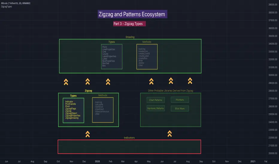
Chart Info & Signature## Overview
Chart Info & Signature displays customizable information tables on your TradingView chart. It consists of two independent tables that can be positioned anywhere on the chart and fully customized to match your branding and preferences.
---
## Table 1: Market Info Table
### What It Displays
The Market Info Table shows essential trading information:
1. **Exchange** - The exchange name (e.g., "BINANCE", "NASDAQ")
2. **Trading Pair** - The symbol pair (e.g., "BTC/USD", "EUR/USD") with optional timeframe
3. **Date** - Current date in DD/MM/YYYY format
4. **Signature** (optional) - Custom text that appears below the date
### Positioning
- **Vertical Position**: Top, Middle, or Bottom of the chart
- **Horizontal Position**: Left, Center, or Right of the chart
- **Exchange Position**: Can be placed at the top or bottom of the table
### Customization Options
#### Exchange Settings
- Show/Hide exchange name
- Text size (tiny, small, normal, large, huge, auto)
- Text color
- Background color
- Position (top or bottom of table)
#### Pair Settings
- Pair delimiter (default: "/")
- Text size
- Text color
- Background color
#### Timeframe Settings
- Show/Hide timeframe (displays current chart timeframe like "1h", "15m", "1D")
#### Date Settings
- Show/Hide date
- Text size
- Text color
- Background color
#### Signature Settings (Below Date)
- Show/Hide signature
- Custom text
- Text size
- Text color
- Background color
- Spacing before signature (with adjustable size)
---
## Table 2: Signature Table
### What It Displays
The Signature Table displays up to 3 customizable text lines, perfect for contact information or any custom text you want to display.
### Positioning
- **Vertical Position**: Top, Middle, or Bottom of the chart
- **Horizontal Position**: Left, Center, or Right of the chart
### Customization Options
#### Line 1 (Top Line)
- Show/Hide line
- Custom text
- Text size
- Text color
- Background color
- Spacing after line (with adjustable size)
#### Line 2 (Middle Line)
- Show/Hide line
- Custom text
- Text size
- Text color
- Background color
- Spacing after line (with adjustable size)
#### Line 3 (Bottom Line)
- Show/Hide line
- Custom text
- Text size
- Text color
- Background color
### Smart Positioning
The table automatically adjusts the spacing between lines based on which lines are visible, ensuring proper alignment regardless of which lines you choose to display.
---
## Key Features
### ✅ Fully Customizable
- Every element can be shown or hidden
- Individual text sizes for each element
- Custom colors for text and backgrounds
- Adjustable spacing between elements
### ✅ Flexible Positioning
- Each table can be positioned independently
- 9 possible positions per table (3 vertical × 3 horizontal)
- Tables can overlap or be placed separately
### ✅ Organized Settings
- Settings are organized into logical groups and subgroups
- Easy to find and modify specific elements
- Clean, intuitive settings panel
### ✅ Dynamic Content
- Trading pair automatically updates based on chart symbol
- Timeframe automatically matches current chart timeframe
- Date updates in real-time
- Exchange name pulled from symbol information
---
## Text Size Options
All text size settings support the following options:
- **tiny** - Smallest fixed size
- **small** - Small fixed size
- **normal** - Standard fixed size
- **large** - Large fixed size
- **huge** - Largest fixed size
- **auto** - Automatically adjusts based on chart zoom and screen size
---
## Default Configuration
- **Market Info Table**: Positioned at top-right, showing exchange, pair with timeframe, and date. Signature row in Market Info Table is hidden by default.
- **Signature Table**: Positioned at bottom-right, showing 3 signature lines with added spacing between line 1 and line 2
- All text uses semi-transparent white (#ffffff77) by default
- All backgrounds are transparent by default
---
## Tips
1. Use **auto** text size for elements that need to scale with chart zoom
2. Use transparent backgrounds for a clean, minimal look
3. Position tables in corners to avoid interfering with price action
4. Customize colors to match your chart theme
5. Hide elements you don't need to keep the display clean

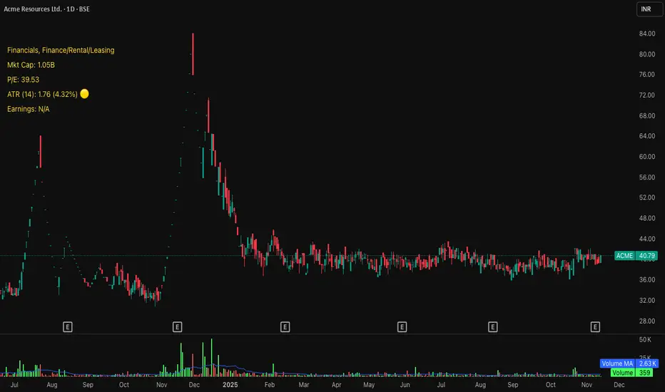
Michael's Custom Watermark🔷 MICHAEL'S CUSTOM WATERMARK INDICATOR
━━━━━━━━━━━━━━━━━━━━━━━━━━━━━━━━━━━━━━━
📊 OVERVIEW
A comprehensive chart watermark overlay that displays essential fundamental and technical information for stocks in a clean, customizable table format. Perfect for traders who want quick access to key metrics without cluttering their charts.
━━━━━━━━━━━━━━━━━━━━━━━━━━━━━━━━━━━━━━━
✨ KEY FEATURES
📊 Fundamental Data Display — Shows Industry, Sector, Market Cap, and P/E Ratio
📅 Earnings Information — Displays next earnings date with countdown timer
📈 ATR Volatility Indicator — 14-day ATR with color-coded visual alerts (🔴🟡🟢)
🎨 Auto Theme Detection — Automatically adjusts text color based on chart background
⚙️ Fully Customizable — Position, colors, size, and displayed metrics all adjustable
🏢 GICS Sector Mapping — Heuristic-based sector classification aligned with industry standards
━━━━━━━━━━━━━━━━━━━━━━━━━━━━━━━━━━━━━━━
🎯 WHAT MAKES THIS INDICATOR UNIQUE?
Unlike basic watermarks, this indicator provides:
Real-time fundamental data integration
Smart theme-aware color adaptation for both light and dark charts
Configurable volatility alerts using ATR thresholds
Earnings countdown feature to never miss important dates
Optimized display that only shows relevant data for the current symbol type
━━━━━━━━━━━━━━━━━━━━━━━━━━━━━━━━━━━━━━━
📖 HOW TO USE
1. BASIC SETUP
Add the indicator to your chart. By default, it displays in the top-left corner with all features enabled.
2. POSITIONING
Vertical Location: Top, Middle, or Bottom
Horizontal Location: Left, Center, or Right
Vertical Offset: Fine-tune position with 0-50 pixel offset from top
3. CUSTOMIZATION OPTIONS
TEXT APPEARANCE:
Auto Text Color — Enable to automatically adapt text color to your chart theme
Manual Color — Set a fixed text color if auto-color is disabled
Text Size — Choose from Huge, Large, Normal, or Small
Theme Colors — Customize text color for light and dark backgrounds separately
DATA DISPLAY TOGGLES:
Show Industry & Sector — Display heuristic-based GICS-aligned sector and industry classification
Show Market Cap — View market capitalization in T/B/M format
Show P/E Ratio — Display Price-to-Earnings ratio (stocks only)
Show ATR (14-Day) — Display Average True Range with percentage and visual indicator
Show Next Earnings — Display upcoming earnings information
Show Earnings Countdown — Show days remaining until next earnings (requires earnings display)
4. ATR VOLATILITY ALERTS
Configure custom thresholds to monitor volatility:
Red Threshold — ATR percentage that triggers red alert 🔴 (default: 6%)
Yellow Threshold — ATR percentage that triggers yellow alert 🟡 (default: 3%)
Green — Shows automatically when ATR is below yellow threshold 🟢
━━━━━━━━━━━━━━━━━━━━━━━━━━━━━━━━━━━━━━━
📐 UNDERSTANDING THE DISPLAY
🏢 SECTOR & INDUSTRY
Shows the GICS sector classification followed by the specific industry. The indicator uses heuristic-based mapping to align TradingView sectors with standard GICS classifications. Note that this mapping is based on keyword detection and industry analysis, so while generally accurate, it may not perfectly match official GICS classifications in all cases.
💰 MARKET CAP
Displays market capitalization using standard abbreviations:
T = Trillion
B = Billion
M = Million
📊 P/E RATIO
Shows the trailing twelve-month Price-to-Earnings ratio. Only displayed for stocks when enabled. Shows "N/A" if data is unavailable.
📈 ATR (14-DAY)
Displays the 14-period Average True Range in both absolute value and percentage terms, with a color-coded indicator:
🔴 Red: High volatility (above red threshold)
🟡 Yellow: Moderate volatility (between yellow and red thresholds)
🟢 Green: Low volatility (below yellow threshold)
📅 EARNINGS
Shows earnings information in three formats:
"X days remaining" — When countdown is enabled and earnings date is known
"Upcoming" — When date is in the future but countdown is disabled
"Recently Reported" — When earnings just occurred
"N/A" — When no earnings data is available
━━━━━━━━━━━━━━━━━━━━━━━━━━━━━━━━━━━━━━━
⚙️ TECHNICAL DETAILS
SUPPORTED INSTRUMENTS:
Optimized for stocks with full fundamental data
Works with other instruments (crypto, forex, futures) but only displays applicable metrics
Automatically suppresses irrelevant data (e.g., P/E for non-stocks)
PERFORMANCE:
Lightweight overlay with minimal resource usage
Updates only on last bar for efficiency
No historical recalculation needed
COMPATIBILITY:
Pine Script v6
Works on all timeframes
Compatible with all chart types
Auto-adapts to theme changes
━━━━━━━━━━━━━━━━━━━━━━━━━━━━━━━━━━━━━━━
💡 TIPS & BEST PRACTICES
Enable Auto Text Color for seamless theme switching between light and dark modes
Adjust vertical offset to avoid overlap with price action in high-volatility periods
Use ATR thresholds appropriate to your trading style and asset class
Disable features you don't use to keep the watermark clean and focused
Position in corners to maximize chart viewing space
Use smaller text size for multi-panel layouts
━━━━━━━━━━━━━━━━━━━━━━━━━━━━━━━━━━━━━━━
🔧 TROUBLESHOOTING
"N/A" SHOWING FOR P/E RATIO:
This is normal for non-stock instruments
May occur for stocks with negative earnings
Check if fundamental data is available for the symbol
EARNINGS SHOWING "N/A":
Earnings data may not be available for all stocks
Check TradingView's data coverage for your symbol
TEXT COLOR NOT VISIBLE:
Enable Auto Text Color feature
Manually set text color to contrast with your chart background
Adjust custom light/dark text colors in settings
━━━━━━━━━━━━━━━━━━━━━━━━━━━━━━━━━━━━━━━
⚠️ DISCLAIMER
This indicator is for informational purposes only. The fundamental data displayed is sourced from TradingView's data providers. Always verify critical information before making trading decisions. Past performance is not indicative of future results.
━━━━━━━━━━━━━━━━━━━━━━━━━━━━━━━━━━━━━━━
If you find this indicator helpful, please give it a boost 🚀 and share your feedback in the comments!
Version: 1.0
Pine Script Version: v6
Created by: Michael
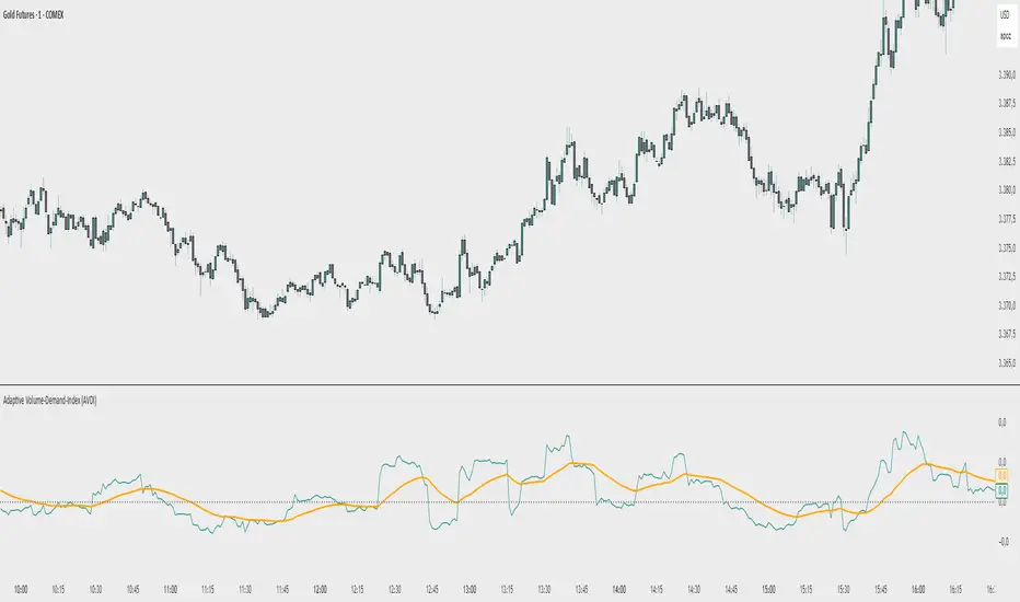
Adaptive Volume‐Demand‐Index (AVDI)Demand Index (according to James Sibbet) – Short Description
The Demand Index (DI) was developed by James Sibbet to measure real “buying” vs. “selling” strength (Demand vs. Supply) using price and volume data. It is not a standalone trading signal, but rather a filter and trend confirmer that should always be used together with chart structure and additional indicators.
---
\ 1. Calculation Basis\
1. Volume Normalization
$$
\text{normVol}_t
= \frac{\text{Volume}_t}{\mathrm{EMA}(\text{Volume},\,n_{\text{Vol}})_t}
\quad(\text{e.g., }n_{\text{Vol}} = 13)
$$
This smooths out extremely high volume spikes and compares them to the average (≈ 1 means “average volume”).
2. Price Factor
$$
\text{priceFactor}_t
= \frac{\text{Close}_t - \text{Open}_t}{\text{Open}_t}.
$$
Positive values for bullish bars, negative for bearish bars.
3. Component per Bar
$$
\text{component}_t
= \text{normVol}_t \times \text{priceFactor}_t.
$$
If volume is above average (> 1) and the price rises slightly, this yields a noticeably positive value; conversely if the price falls.
4. Raw DI (Rolling Sum)
Over a window of \$w\$ bars (e.g., 20):
$$
\text{RawDI}_t
= \sum_{i=0}^{w-1} \text{component}_{\,t-i}.
$$
Alternatively, recursively for \$t \ge w\$:
$$
\text{RawDI}_t
= \text{RawDI}_{t-1}
+ \text{component}_t
- \text{component}_{\,t-w}.
$$
5. Optional EMA Smoothing
An EMA over RawDI (e.g., \$n\_{\text{DI}} = 50\$) reduces short-term fluctuations and highlights medium-term trends:
$$
\text{EMA\_DI}_t
= \mathrm{EMA}(\text{RawDI},\,n_{\text{DI}})_t.
$$
6.Zero Line
Handy guideline:
RawDI > 0: Accumulated buying power dominates.
RawDI < 0: Accumulated selling power dominates.
2. Interpretation & Application
Crossing Zero
RawDI above zero → Indication of increasing buying pressure (potential long signal).
RawDI below zero → Indication of increasing selling pressure (potential short signal).
Not to be used alone for entry—always confirm with price action.
RawDI vs. EMA_DI
RawDI > EMA\_DI → Acceleration of demand.
RawDI < EMA\_DI → Weakening of demand.
Divergences
Price makes a new high, RawDI does not make a higher high → potential weakness in the uptrend.
Price makes a new low, RawDI does not make a lower low → potential exhaustion of the downtrend.
3. Typical Signals (for Beginners)
\ 1. Long Setup\
RawDI crosses zero from below,
RawDI > EMA\_DI (acceleration),
Price closes above a short-term swing high or resistance.
Stop-Loss: just below the last swing low, Take-Profit/Trailing: on reversal signals or fixed R\:R.
2. Short Setup
RawDI crosses zero from above,
RawDI < EMA\_DI (increased selling pressure),
Price closes below a short-term swing low or support.
Stop-Loss: just above the last swing high.
---
4. Notes and Parameters
Recommended Values (Beginners):
Volume EMA (n₍Vol₎) = 13
RawDI window (w) = 20
EMA over DI (n₍DI₎) = 50 (medium-term) or 1 (no smoothing)
Attention:\
NEVER use in isolation. Always in combination with price action analysis (trendlines, support/resistance, candlestick patterns).
Especially during volatile news phases, RawDI can fluctuate strongly → EMA\_DI helps to avoid false signals.
---
Conclusion The Demand Index by James Sibbet is a powerful filter to assess price movements by their volume backing. It shows whether a rally is truly driven by demand or merely a short-term volume anomaly. In combination with classic chart analysis and risk management, it helps to identify robust entry points and potential trend reversals earlier.
ADR% Extension Levels from SMA 50I created this indicator inspired by RealSimpleAriel (a swing trader I recommend following on X) who does not buy stocks extended beyond 4 ADR% from the 50 SMA and uses extensions from the 50 SMA at 7-8-9-10-11-12-13 ADR% to take profits with a 20% position trimming.
RealSimpleAriel's strategy (as I understood it):
-> Focuses on leading stocks from leading groups and industries, i.e., those that have grown the most in the last 1-3-6 months (see on Finviz groups and then select sector-industry).
-> Targets stocks with the best technical setup for a breakout, above the 200 SMA in a bear market and above both the 50 SMA and 200 SMA in a bull market, selecting those with growing Earnings and Sales.
-> Buys stocks on breakout with a stop loss set at the day's low of the breakout and ensures they are not extended beyond 4 ADR% from the 50 SMA.
-> 3-5 day momentum burst: After a breakout, takes profits by selling 1/2 or 1/3 of the position after a 3-5 day upward move.
-> 20% trimming on extension from the 50 SMA: At 7 ADR% (ADR% calculated over 20 days) extension from the 50 SMA, takes profits by selling 20% of the remaining position. Continues to trim 20% of the remaining position based on the stock price extension from the 50 SMA, calculated using the 20-period ADR%, thus trimming 20% at 8-9-10-11 ADR% extension from the 50 SMA. Upon reaching 12-13 ADR% extension from the 50 SMA, considers the stock overextended, closes the remaining position, and evaluates a short.
-> Trailing stop with ascending SMA: Uses a chosen SMA (10, 20, or 50) as the definitive stop loss for the position, depending on the stock's movement speed (preferring larger SMAs for slower-moving stocks or for long-term theses). If the stock's closing price falls below the chosen SMA, the entire position is closed.
In summary:
-->Buy a breakout using the day's low of the breakout as the stop loss (this stop loss is the most critical).
--> Do not buy stocks extended beyond 4 ADR% from the 50 SMA.
--> Sell 1/2 or 1/3 of the position after 3-5 days of upward movement.
--> Trim 20% of the position at each 7-8-9-10-11-12-13 ADR% extension from the 50 SMA.
--> Close the entire position if the breakout fails and the day's low of the breakout is reached.
--> Close the entire position if the price, during the rise, falls below a chosen SMA (10, 20, or 50, depending on your preference).
--> Definitively close the position if it reaches 12-13 ADR% extension from the 50 SMA.
I used Grok from X to create this indicator. I am not a programmer, but based on the ADR% I use, it works.
Below is Grok from X's description of the indicator:
Script Description
The script is a custom indicator for TradingView that displays extension levels based on ADR% relative to the 50-period Simple Moving Average (SMA). Below is a detailed description of its features, structure, and behavior:
1. Purpose of the Indicator
Name: "ADR% Extension Levels from SMA 50".
Objective: Draw horizontal blue lines above and below the 50-period SMA, corresponding to specific ADR% multiples (4, 7, 8, 9, 10, 11, 12, 13). These levels represent potential price extension zones based on the average daily percentage volatility.
Overlay: The indicator is overlaid on the price chart (overlay=true), so the lines and SMA appear directly on the price graph.
2. Configurable Inputs
The indicator allows users to customize parameters through TradingView settings:
SMA Length (smaLength):
Default: 50 periods.
Description: Specifies the number of periods for calculating the Simple Moving Average (SMA). The 50-period SMA serves as the reference point for extension levels.
Constraint: Minimum 1 period.
ADR% Length (adrLength):
Default: 20 periods.
Description: Specifies the number of days to calculate the moving average of the daily high/low ratio, used to determine ADR%.
Constraint: Minimum 1 period.
Scale Factor (scaleFactor):
Default: 1.0.
Description: An optional multiplier to adjust the distance of extension levels from the SMA. Useful if levels are too close or too far due to an overly small or large ADR%.
Constraint: Minimum 0.1, increments of 0.1.
Tooltip: "Adjust if levels are too close or far from SMA".
3. Main Calculations
50-period SMA:
Calculated with ta.sma(close, smaLength) using the closing price (close).
Serves as the central line around which extension levels are drawn.
ADR% (Average Daily Range Percentage):
Formula: 100 * (ta.sma(dhigh / dlow, adrLength) - 1).
Details:
dhigh and dlow are the daily high and low prices, obtained via request.security(syminfo.tickerid, "D", high/low) to ensure data is daily-based, regardless of the chart's timeframe.
The dhigh / dlow ratio represents the daily percentage change.
The simple moving average (ta.sma) of this ratio over 20 days (adrLength) is subtracted by 1 and multiplied by 100 to obtain ADR% as a percentage.
The result is multiplied by scaleFactor for manual adjustments.
Extension Levels:
Defined as ADR% multiples: 4, 7, 8, 9, 10, 11, 12, 13.
Stored in an array (levels) for easy iteration.
For each level, prices above and below the SMA are calculated as:
Above: sma50 * (1 + (level * adrPercent / 100))
Below: sma50 * (1 - (level * adrPercent / 100))
These represent price levels corresponding to a percentage change from the SMA equal to level * ADR%.
4. Visualization
Horizontal Blue Lines:
For each level (4, 7, 8, 9, 10, 11, 12, 13 ADR%), two lines are drawn:
One above the SMA (e.g., +4 ADR%).
One below the SMA (e.g., -4 ADR%).
Color: Blue (color.blue).
Style: Solid (style=line.style_solid).
Management:
Each level has dedicated variables for upper and lower lines (e.g., upperLine1, lowerLine1 for 4 ADR%).
Previous lines are deleted with line.delete before drawing new ones to avoid overlaps.
Lines are updated at each bar with line.new(bar_index , level, bar_index, level), covering the range from the previous bar to the current one.
Labels:
Displayed only on the last bar (barstate.islast) to avoid clutter.
For each level, two labels:
Above: E.g., "4 ADR%", positioned above the upper line (style=label.style_label_down).
Below: E.g., "-4 ADR%", positioned below the lower line (style=label.style_label_up).
Color: Blue background, white text.
50-period SMA:
Drawn as a gray line (color.gray) for visual reference.
Diagnostics:
ADR% Plot: ADR% is plotted in the status line (orange, histogram style) to verify the value.
ADR% Label: A label on the last bar near the SMA shows the exact ADR% value (e.g., "ADR%: 2.34%"), with a gray background and white text.
5. Behavior
Dynamic Updating:
Lines update with each new bar to reflect new SMA 50 and ADR% values.
Since ADR% uses daily data ("D"), it remains constant within the same day but changes day-to-day.
Visibility Across All Bars:
Lines are drawn on every bar, not just the last one, ensuring visibility on historical data as well.
Adaptability:
The scaleFactor allows level adjustments if ADR% is too small (e.g., for low-volatility symbols) or too large (e.g., for cryptocurrencies).
Compatibility:
Works on any timeframe since ADR% is calculated from daily data.
Suitable for symbols with varying volatility (e.g., stocks, forex, cryptocurrencies).
6. Intended Use
Technical Analysis: Extension levels represent significant price zones based on average daily volatility. They can be used to:
Identify potential price targets (e.g., take profit at +7 ADR%).
Assess support/resistance zones (e.g., -4 ADR% as support).
Measure price extension relative to the 50 SMA.
Trading: Useful for strategies based on breakouts or mean reversion, where ADR% levels indicate reversal or continuation points.
Debugging: Labels and ADR% plot help verify that values align with the symbol’s volatility.
7. Limitations
Dependence on Daily Data: ADR% is based on daily dhigh/dlow, so it may not reflect intraday volatility on short timeframes (e.g., 1 minute).
Extreme ADR% Values: For low-volatility symbols (e.g., bonds) or high-volatility symbols (e.g., meme stocks), ADR% may require adjustments via scaleFactor.
Graphical Load: Drawing 16 lines (8 upper, 8 lower) on every bar may slow the chart for very long historical periods, though line management is optimized.
ADR% Formula: The formula 100 * (sma(dhigh/dlow, Length) - 1) may produce different values compared to other ADR% definitions (e.g., (high - low) / close * 100), so users should be aware of the context.
8. Visual Example
On a chart of a stock like TSLA (daily timeframe):
The 50 SMA is a gray line tracking the average trend.
Assuming an ADR% of 3%:
At +4 ADR% (12%), a blue line appears at sma50 * 1.12.
At -4 ADR% (-12%), a blue line appears at sma50 * 0.88.
Other lines appear at ±7, ±8, ±9, ±10, ±11, ±12, ±13 ADR%.
On the last bar, labels show "4 ADR%", "-4 ADR%", etc., and a gray label shows "ADR%: 3.00%".
ADR% is visible in the status line as an orange histogram.
9. Code: Technical Structure
Language: Pine Script @version=5.
Inputs: Three configurable parameters (smaLength, adrLength, scaleFactor).
Calculations:
SMA: ta.sma(close, smaLength).
ADR%: 100 * (ta.sma(dhigh / dlow, adrLength) - 1) * scaleFactor.
Levels: sma50 * (1 ± (level * adrPercent / 100)).
Graphics:
Lines: Created with line.new, deleted with line.delete to avoid overlaps.
Labels: Created with label.new only on the last bar.
Plots: plot(sma50) for the SMA, plot(adrPercent) for debugging.
Optimization: Uses dedicated variables for each line (e.g., upperLine1, lowerLine1) for clear management and to respect TradingView’s graphical object limits.
10. Possible Improvements
Option to show lines only on the last bar: Would reduce visual clutter.
Customizable line styles: Allow users to choose color or style (e.g., dashed).
Alert for anomalous ADR%: A message if ADR% is too small or large.
Dynamic levels: Allow users to specify ADR% multiples via input.
Optimization for short timeframes: Adapt ADR% for intraday timeframes.
Conclusion
The script creates a visual indicator that helps traders identify price extension levels based on daily volatility (ADR%) relative to the 50 SMA. It is robust, configurable, and includes debugging tools (ADR% plot and labels) to verify values. The ADR% formula based on dhigh/dlow

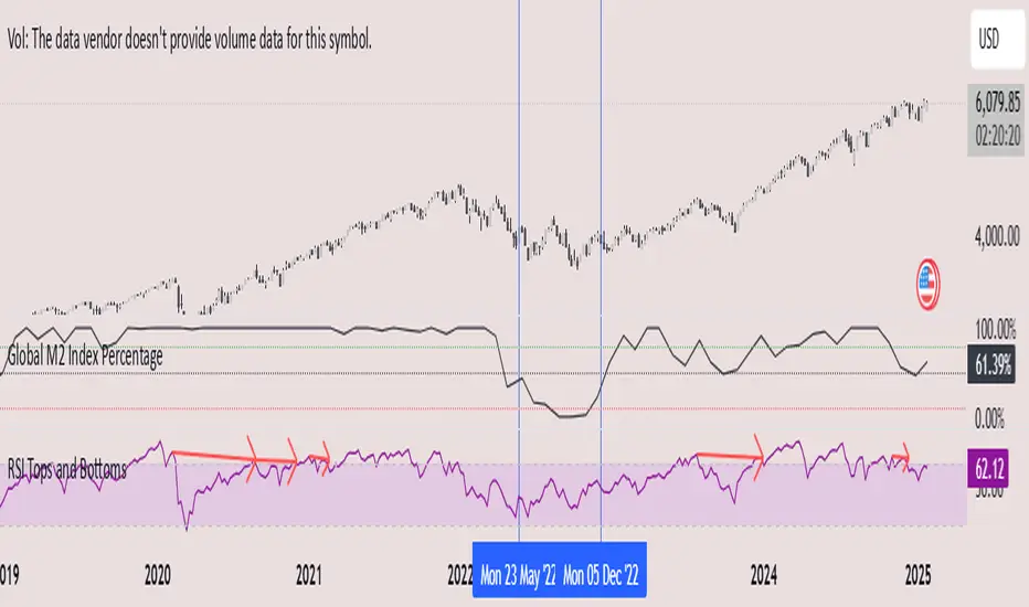
Global M2 Index Percentage### **Global M2 Index Percentage**
**Description:**
The **Global M2 Index Percentage** is a custom indicator designed to track and visualize the global money supply (M2) in a normalized percentage format. It aggregates M2 data from major economies (e.g., the US, EU, China, Japan, and the UK) and adjusts for exchange rates to provide a comprehensive view of global liquidity. This indicator helps traders and investors understand the broader macroeconomic environment, identify trends in money supply, and make informed decisions based on global liquidity conditions.
---
### **How It Works:**
1. **Data Aggregation**:
- The indicator collects M2 data from key economies and adjusts it using exchange rates to calculate a global M2 value.
- The formula for global M2 is:
\
2. **Normalization**:
- The global M2 value is normalized into a percentage (0% to 100%) based on its range over a user-defined period (default: 13 weeks).
- The formula for normalization is:
\
3. **Visualization**:
- The indicator plots the M2 Index as a line chart.
- Key reference levels are highlighted:
- **10% (Red Line)**: Oversold level (low liquidity).
- **50% (Black Line)**: Neutral level.
- **80% (Green Line)**: Overbought level (high liquidity).
---
### **How to Use the Indicator:**
#### **1. Understanding the M2 Index:**
- **Below 10%**: Indicates extremely low liquidity, which may signal economic contraction or tight monetary policy.
- **Above 80%**: Indicates high liquidity, which may signal loose monetary policy or potential inflationary pressures.
- **Between 10% and 80%**: Represents a neutral to moderate liquidity environment.
#### **2. Trading Strategies:**
- **Long-Term Investing**:
- Use the M2 Index to assess global liquidity trends.
- **High M2 Index (e.g., >80%)**: Consider investing in risk assets (stocks, commodities) as liquidity supports growth.
- **Low M2 Index (e.g., <10%)**: Shift to defensive assets (bonds, gold) as liquidity tightens.
- **Short-Term Trading**:
- Combine the M2 Index with technical indicators (e.g., RSI, MACD) for timing entries and exits.
- **M2 Index Rising + RSI Oversold**: Potential buying opportunity.
- **M2 Index Falling + RSI Overbought**: Potential selling opportunity.
#### **3. Macroeconomic Analysis**:
- Use the M2 Index to monitor the impact of central bank policies (e.g., quantitative easing, rate hikes).
- Correlate the M2 Index with inflation data (CPI, PPI) to anticipate inflationary or deflationary trends.
---
### **Key Features:**
- **Customizable Timeframe**: Adjust the lookback period (e.g., 13 weeks, 26 weeks) to suit your trading style.
- **Multi-Economy Data**: Aggregates M2 data from the US, EU, China, Japan, and the UK for a global perspective.
- **Normalized Output**: Converts raw M2 data into an easy-to-interpret percentage format.
- **Reference Levels**: Includes key levels (10%, 50%, 80%) for quick analysis.
---
### **Example Use Case:**
- **Scenario**: The M2 Index rises from 49% to 62% over two weeks.
- **Interpretation**: Global liquidity is increasing, potentially due to central bank stimulus.
- **Action**:
- **Long-Term**: Increase exposure to equities and commodities.
- **Short-Term**: Look for buying opportunities in oversold assets (e.g., RSI < 30).
---
### **Why Use the Global M2 Index Percentage?**
- **Macro Insights**: Understand the broader economic environment and its impact on financial markets.
- **Risk Management**: Identify periods of high or low liquidity to adjust your portfolio accordingly.
- **Enhanced Timing**: Combine with technical analysis for better entry and exit points.
---
### **Conclusion:**
The **Global M2 Index Percentage** is a powerful tool for traders and investors seeking to incorporate macroeconomic data into their strategies. By tracking global liquidity trends, this indicator helps you make informed decisions, whether you're trading short-term or planning long-term investments. Add it to your TradingView charts today and gain a deeper understanding of the global money supply!
---
**Disclaimer**: This indicator is for informational purposes only and should not be considered financial advice. Always conduct your own research and consult with a professional before making investment decisions.
Visible and Anchored OTE chart [SYNC & TRADE]Thanks for the start @twingall
Visible and Anchored OTE chart
Indicator for visualizing price levels and optimal trading zones (OTE - Optimal Trading Entry) using Fibonacci levels.
Main features
Visualization of price ranges using two OTE zones:
OTE 70% (79-62 Fibonacci levels)
OTE 30% (21-38 Fibonacci levels)
Setting up time periods:
Ability to use a custom date range
Option to work with a higher time frame
Flexible display settings:
Choose between using candle bodies or the full range for binding
Customizable appearance of OTE boxes
Customizable text labels
Additional levels:
Middle line (50.5%)
Optional levels of 29.5%, 70.5% and 88%
Customizable Fibonacci extensions
Indicator settings
Main parameters
Use Custom Dates - enable a custom date range
Start Date/End Date - set a time range
Use Higher Timeframe - use a higher time frame
Higher Timeframe - select a higher timeframe
Setting up OTE zones
Show Fib Box - displaying OTE zones
Enable Fib Box 79-62 - enabling OTE zone 70%
Enable Fib Box 21-38 - enabling OTE zone 30%
Show Text - displaying text labels in zones
Visual design
Text Size - text size (tiny/small/medium/large)
Text Color - text color
Text Alignment - text alignment
Line Thickness - line thickness (1-4)
Line Style - line style (Solid/Dashed/Dotted)
Fibonacci levels
High/Low Lines - displaying extreme levels
Midline - displaying the middle line (50.5%)
Show 29.5 Line - additional level 29.5%
Show 70.5 Line - additional level 70.5%
Show 88 Line - additional level 88%
Extensions Fibonacci
There are 6 customizable extension levels available:
Ext#1 (default 1.0)
Ext#2 (default 1.27)
Ext#3 (default 1.62)
Ext#4 (default 2.0)
Ext#5 (default 2.62)
Ext#6 (default 3.62)
For each level, you can configure:
On/Off
Color
Meaning
Alerts
The indicator provides the following types of alerts:
Entering/Exiting OTE Zones:
Entering 70% OTE Zone
Exiting 70% OTE Zone
Entering 30% OTE Zone
Exiting 30% OTE Zone
Crossing Additional Levels:
Crossing 29.5% Level
Crossing 70.5% Level
Crossing 88% Level
Reaching Extension Levels Fibonacci:
Alerts for each configured extension level
Support for both positive and negative extensions
Usage
Add the indicator to the chart
Configure the required display parameters
Set alerts if necessary
Use OTE zones to identify potential entry points into the market
Notes
The indicator automatically updates when the visible area of the chart changes
When using a custom date range, make sure the selected period contains data
For correct operation with a higher time frame, make sure that historical data is available
Visible and Anchored OTE chart
Индикатор для визуализации ценовых уровней и зон оптимальной торговли (OTE - Optimal Trading Entry) с использованием уровней Фибоначчи.
Основные возможности
Визуализация ценовых диапазонов с помощью двух OTE зон:
OTE 70% (79-62 уровни Фибоначчи)
OTE 30% (21-38 уровни Фибоначчи)
Настройка временных периодов:
Возможность использования пользовательского диапазона дат
Опция работы с высшим таймфреймом
Гибкая настройка отображения:
Выбор между использованием тел свечей или полного диапазона для привязки
Настраиваемый внешний вид боксов OTE
Настраиваемые текстовые метки
Дополнительные уровни:
Средняя линия (50.5%)
Опциональные уровни 29.5%, 70.5% и 88%
Настраиваемые расширения Фибоначчи
Настройка индикатора
Основные параметры
Use Custom Dates - включение пользовательского диапазона дат
Start Date/End Date - установка временного диапазона
Use Higher Timeframe - использование высшего таймфрейма
Higher Timeframe - выбор высшего таймфрейма
Настройка OTE зон
Show Fib Box - отображение зон OTE
Enable Fib Box 79-62 - включение зоны OTE 70%
Enable Fib Box 21-38 - включение зоны OTE 30%
Show Text - отображение текстовых меток в зонах
Визуальное оформление
Text Size - размер текста (tiny/small/medium/large)
Text Color - цвет текста
Text Alignment - выравнивание текста
Line Thickness - толщина линий (1-4)
Line Style - стиль линий (Solid/Dashed/Dotted)
Уровни Фибоначчи
High/Low Lines - отображение крайних уровней
Midline - отображение средней линии (50.5%)
Show 29.5 Line - дополнительный уровень 29.5%
Show 70.5 Line - дополнительный уровень 70.5%
Show 88 Line - дополнительный уровень 88%
Расширения Фибоначчи
Доступно 6 настраиваемых уровней расширения:
Ext#1 (по умолчанию 1.0)
Ext#2 (по умолчанию 1.27)
Ext#3 (по умолчанию 1.62)
Ext#4 (по умолчанию 2.0)
Ext#5 (по умолчанию 2.62)
Ext#6 (по умолчанию 3.62)
Для каждого уровня можно настроить:
Включение/выключение
Цвет
Значение
Оповещения
Индикатор предоставляет следующие типы оповещений:
Вход/выход из зон OTE:
Вход в зону OTE 70%
Выход из зоны OTE 70%
Вход в зону OTE 30%
Выход из зоны OTE 30%
Пересечение дополнительных уровней:
Пересечение уровня 29.5%
Пересечение уровня 70.5%
Пересечение уровня 88%
Достижение уровней расширения Фибоначчи:
Оповещения для каждого настроенного уровня расширения
Поддержка как положительных, так и отрицательных расширений
Использование
Добавьте индикатор на график
Настройте необходимые параметры отображения
При необходимости установите оповещения
Используйте зоны OTE для определения потенциальных точек входа в рынок
Примечания
Индикатор автоматически обновляется при изменении видимой области графика
При использовании пользовательского диапазона дат убедитесь, что выбранный период содержит данные
Для корректной работы с высшим таймфреймом убедитесь в доступности исторических данных
analytics_tablesLibrary "analytics_tables"
📝 Description
This library provides the implementation of several performance-related statistics and metrics, presented in the form of tables.
The metrics shown in the afforementioned tables where developed during the past years of my in-depth analalysis of various strategies in an atempt to reason about the performance of each strategy.
The visualization and some statistics where inspired by the existing implementations of the "Seasonality" script, and the performance matrix implementations of @QuantNomad and @ZenAndTheArtOfTrading scripts.
While this library is meant to be used by my strategy framework "Template Trailing Strategy (Backtester)" script, I wrapped it in a library hoping this can be usefull for other community strategy scripts that will be released in the future.
🤔 How to Guide
To use the functionality this library provides in your script you have to import it first!
Copy the import statement of the latest release by pressing the copy button below and then paste it into your script. Give a short name to this library so you can refer to it later on. The import statement should look like this:
import jason5480/analytics_tables/1 as ant
There are three types of tables provided by this library in the initial release. The stats table the metrics table and the seasonality table.
Each one shows different kinds of performance statistics.
The table UDT shall be initialized once using the `init()` method.
They can be updated using the `update()` method where the updated data UDT object shall be passed.
The data UDT can also initialized and get updated on demend depending on the use case
A code example for the StatsTable is the following:
var ant.StatsData statsData = ant.StatsData.new()
statsData.update(SideStats.new(), SideStats.new(), 0)
if (barstate.islastconfirmedhistory or (barstate.isrealtime and barstate.isconfirmed))
var statsTable = ant.StatsTable.new().init(ant.getTablePos('TOP', 'RIGHT'))
statsTable.update(statsData)
A code example for the MetricsTable is the following:
var ant.StatsData statsData = ant.StatsData.new()
statsData.update(ant.SideStats.new(), ant.SideStats.new(), 0)
if (barstate.islastconfirmedhistory or (barstate.isrealtime and barstate.isconfirmed))
var metricsTable = ant.MetricsTable.new().init(ant.getTablePos('BOTTOM', 'RIGHT'))
metricsTable.update(statsData, 10)
A code example for the SeasonalityTable is the following:
var ant.SeasonalData seasonalData = ant.SeasonalData.new().init(Seasonality.monthOfYear)
seasonalData.update()
if (barstate.islastconfirmedhistory or (barstate.isrealtime and barstate.isconfirmed))
var seasonalTable = ant.SeasonalTable.new().init(seasonalData, ant.getTablePos('BOTTOM', 'LEFT'))
seasonalTable.update(seasonalData)
🏋️♂️ Please refer to the "EXAMPLE" regions of the script for more advanced and up to date code examples!
Special thanks to @Mrcrbw for the proposal to develop this library and @DCNeu for the constructive feedback 🏆.
getTablePos(ypos, xpos)
Get table position compatible string
Parameters:
ypos (simple string) : The position on y axise
xpos (simple string) : The position on x axise
Returns: The position to be passed to the table
method init(this, pos, height, width, positiveTxtColor, negativeTxtColor, neutralTxtColor, positiveBgColor, negativeBgColor, neutralBgColor)
Initialize the stats table object with the given colors in the given position
Namespace types: StatsTable
Parameters:
this (StatsTable) : The stats table object
pos (simple string) : The table position string
height (simple float) : The height of the table as a percentage of the charts height. By default, 0 auto-adjusts the height based on the text inside the cells
width (simple float) : The width of the table as a percentage of the charts height. By default, 0 auto-adjusts the width based on the text inside the cells
positiveTxtColor (simple color) : The text color when positive
negativeTxtColor (simple color) : The text color when negative
neutralTxtColor (simple color) : The text color when neutral
positiveBgColor (simple color) : The background color with transparency when positive
negativeBgColor (simple color) : The background color with transparency when negative
neutralBgColor (simple color) : The background color with transparency when neutral
method init(this, pos, height, width, neutralBgColor)
Initialize the metrics table object with the given colors in the given position
Namespace types: MetricsTable
Parameters:
this (MetricsTable) : The metrics table object
pos (simple string) : The table position string
height (simple float) : The height of the table as a percentage of the charts height. By default, 0 auto-adjusts the height based on the text inside the cells
width (simple float) : The width of the table as a percentage of the charts width. By default, 0 auto-adjusts the width based on the text inside the cells
neutralBgColor (simple color) : The background color with transparency when neutral
method init(this, seas)
Initialize the seasonal data
Namespace types: SeasonalData
Parameters:
this (SeasonalData) : The seasonal data object
seas (simple Seasonality) : The seasonality of the matrix data
method init(this, data, pos, maxNumOfYears, height, width, extended, neutralTxtColor, neutralBgColor)
Initialize the seasonal table object with the given colors in the given position
Namespace types: SeasonalTable
Parameters:
this (SeasonalTable) : The seasonal table object
data (SeasonalData) : The seasonality data of the table
pos (simple string) : The table position string
maxNumOfYears (simple int) : The maximum number of years that fit into the table
height (simple float) : The height of the table as a percentage of the charts height. By default, 0 auto-adjusts the height based on the text inside the cells
width (simple float) : The width of the table as a percentage of the charts width. By default, 0 auto-adjusts the width based on the text inside the cells
extended (simple bool) : The seasonal table with extended columns for performance
neutralTxtColor (simple color) : The text color when neutral
neutralBgColor (simple color) : The background color with transparency when neutral
method update(this, wins, losses, numOfInconclusiveExits)
Update the strategy info data of the strategy
Namespace types: StatsData
Parameters:
this (StatsData) : The strategy statistics object
wins (SideStats)
losses (SideStats)
numOfInconclusiveExits (int) : The number of inconclusive trades
method update(this, stats, positiveTxtColor, negativeTxtColor, negativeBgColor, neutralBgColor)
Update the stats table object with the given data
Namespace types: StatsTable
Parameters:
this (StatsTable) : The stats table object
stats (StatsData) : The stats data to update the table
positiveTxtColor (simple color) : The text color when positive
negativeTxtColor (simple color) : The text color when negative
negativeBgColor (simple color) : The background color with transparency when negative
neutralBgColor (simple color) : The background color with transparency when neutral
method update(this, stats, buyAndHoldPerc, positiveTxtColor, negativeTxtColor, positiveBgColor, negativeBgColor)
Update the metrics table object with the given data
Namespace types: MetricsTable
Parameters:
this (MetricsTable) : The metrics table object
stats (StatsData) : The stats data to update the table
buyAndHoldPerc (float) : The buy and hold percetage
positiveTxtColor (simple color) : The text color when positive
negativeTxtColor (simple color) : The text color when negative
positiveBgColor (simple color) : The background color with transparency when positive
negativeBgColor (simple color) : The background color with transparency when negative
method update(this)
Update the seasonal data based on the season and eon timeframe
Namespace types: SeasonalData
Parameters:
this (SeasonalData) : The seasonal data object
method update(this, data, positiveTxtColor, negativeTxtColor, neutralTxtColor, positiveBgColor, negativeBgColor, neutralBgColor, timeBgColor)
Update the seasonal table object with the given data
Namespace types: SeasonalTable
Parameters:
this (SeasonalTable) : The seasonal table object
data (SeasonalData) : The seasonal cell data to update the table
positiveTxtColor (simple color) : The text color when positive
negativeTxtColor (simple color) : The text color when negative
neutralTxtColor (simple color) : The text color when neutral
positiveBgColor (simple color) : The background color with transparency when positive
negativeBgColor (simple color) : The background color with transparency when negative
neutralBgColor (simple color) : The background color with transparency when neutral
timeBgColor (simple color) : The background color of the time gradient
SideStats
Object that represents the strategy statistics data of one side win or lose
Fields:
numOf (series int)
sumFreeProfit (series float)
freeProfitStDev (series float)
sumProfit (series float)
profitStDev (series float)
sumGain (series float)
gainStDev (series float)
avgQuantityPerc (series float)
avgCapitalRiskPerc (series float)
avgTPExecutedCount (series float)
avgRiskRewardRatio (series float)
maxStreak (series int)
StatsTable
Object that represents the stats table
Fields:
table (series table) : The actual table
rows (series int) : The number of rows of the table
columns (series int) : The number of columns of the table
StatsData
Object that represents the statistics data of the strategy
Fields:
wins (SideStats)
losses (SideStats)
numOfInconclusiveExits (series int)
avgFreeProfitStr (series string)
freeProfitStDevStr (series string)
lossFreeProfitStDevStr (series string)
avgProfitStr (series string)
profitStDevStr (series string)
lossProfitStDevStr (series string)
avgQuantityStr (series string)
MetricsTable
Object that represents the metrics table
Fields:
table (series table) : The actual table
rows (series int) : The number of rows of the table
columns (series int) : The number of columns of the table
SeasonalData
Object that represents the seasonal table dynamic data
Fields:
seasonality (series Seasonality)
eonToMatrixRow (map)
numOfEons (series int)
mostRecentMatrixRow (series int)
balances (matrix)
returnPercs (matrix)
maxDDs (matrix)
eonReturnPercs (array)
eonCAGRs (array)
eonMaxDDs (array)
SeasonalTable
Object that represents the seasonal table
Fields:
table (series table) : The actual table
headRows (series int) : The number of head rows of the table
headColumns (series int) : The number of head columns of the table
eonRows (series int) : The number of eon rows of the table
seasonColumns (series int) : The number of season columns of the table
statsRows (series int)
statsColumns (series int) : The number of stats columns of the table
rows (series int) : The number of rows of the table
columns (series int) : The number of columns of the table
extended (series bool) : Whether the table has additional performance statistics

BooBee Digital - Enhanced Buy & Sell Alerts Suite
BooBee Digital - Enhanced Buy & Sell Alerts Suite
Introduction:
The “BooBee Digital - Enhanced Buy & Sell Alerts Suite” is a comprehensive trading tool designed to provide traders with precise buy and sell signals by integrating the Average True Range (ATR) trailing stop technique and the Volume Weighted Average Price (VWAP) indicator. This script is tailored to help traders make informed decisions by considering both market volatility and trading volume.
How It Works:
1. ATR Calculation:
• Purpose: Measures market volatility to set dynamic stop levels.
• Details: The Average True Range (ATR) is calculated over a user-defined period. The ATR value reflects the average range of price movements over the specified period, which is crucial for assessing market volatility.
2. ATR Trailing Stop:
• Purpose: Identifies potential trend reversals by setting trailing stops based on market volatility.
• Details: The ATR trailing stop is dynamically adjusted using the ATR value and a user-defined sensitivity factor. This trailing stop level helps identify trend reversals by moving in accordance with price fluctuations.
3. VWAP Calculation:
• Purpose: Provides a volume-weighted average price to benchmark fair value.
• Details: The VWAP is calculated by taking the sum of the product of price and volume, divided by the total volume. This indicator gives traders a reference point for the average price at which the asset has traded throughout the day, considering trading volume.
4. EMA Crossover:
• Purpose: Adds a confirmation layer for buy and sell signals.
• Details: A 1-period Exponential Moving Average (EMA) is used to identify short-term price movements. Buy and sell signals are generated based on the crossover of the EMA and the ATR trailing stop, adding an extra layer of confirmation for trade entries and exits.
Signal Generation:
Buy Signal:
• Generated when the price is above the ATR trailing stop and there is a bullish crossover of the EMA and ATR trailing stop.
• Indicator: Green label below the bar with “Buy” text.
Sell Signal:
• Generated when the price is below the ATR trailing stop and there is a bearish crossover of the EMA and ATR trailing stop.
• Indicator: Red label above the bar with “Sell” text.
VWAP Line:
• The VWAP line is plotted on the chart to help traders identify significant price levels based on trading volume.
• Indicator: Blue line representing the VWAP.
How to Use:
• Chart Type: The script is designed for use on standard chart types such as Candlestick and OHLC. It does not support non-standard chart types like Heikin Ashi, Renko, Kagi, Point & Figure, and Range, as they may produce unrealistic results.
• Clean Chart: Ensure your chart is clean and free of other indicators to avoid confusion. The signals and colors plotted by the script should be easily identifiable.
• Trade Confirmation: Use the buy and sell signals generated by the script in conjunction with other analysis methods to confirm trades.
Key Concepts:
• ATR Trailing Stop: This technique sets dynamic stop levels based on market volatility, helping to identify trend reversals.
• VWAP: This indicator provides a benchmark for the average price considering trading volume, helping traders identify fair value.
• EMA Crossover: This adds a layer of confirmation for buy and sell signals, improving the accuracy of trade entries and exits.

IndicatorsLibrary "Indicators"
this has a calculation for the most used indicators.
macd4C(fastMa, slowMa)
this calculates macd 4c
Parameters:
fastMa (simple int) : is the period for the fast ma. the minimum value is 7
slowMa (simple int) : is the period for the slow ma. the minimum value is 7
Returns: the macd 4c value for the current bar
rsi(rsiSourceInput, rsiLengthInput)
this calculates rsi
Parameters:
rsiSourceInput (float) : is the source for the rsi
rsiLengthInput (simple int) : is the period for the rsi
Returns: the rsi value for the current bar
ao(source, fastPeriod, slowPeriod)
this calculates ao
Parameters:
source (float) : is the source for the ao
fastPeriod (int) : is the period for the fast ma
slowPeriod (int) : is the period for the slow ma
Returns: the ao value for the current bar
kernelAoOscillator(kernelFastLookback, kernelSlowLookback, kernelFastWeight, kernelSlowWeight, kernelFastRegressionStart, kernelSlowRegressionStart, kernelFastSmoothPeriod, kernelSlowSmoothPeriod, kernelFastSmooth, kernelSlowSmooth, source)
this calculates our own kernel ao oscillator which we made
Parameters:
kernelFastLookback (simple int)
kernelSlowLookback (simple int)
kernelFastWeight (simple float)
kernelSlowWeight (simple float)
kernelFastRegressionStart (simple int)
kernelSlowRegressionStart (simple int)
kernelFastSmoothPeriod (int)
kernelSlowSmoothPeriod (int)
kernelFastSmooth (bool)
kernelSlowSmooth (bool)
source (float) : is the source for the ao
Returns: the kernel ao oscillator value for the current bar, the colors for both the fast and slow kernel, the fast & slow kernel
signalLineKernel(lag, h, r, x_0, smoothColors, _src, c_bullish, c_bearish)
Parameters:
lag (int)
h (float)
r (float)
x_0 (int)
smoothColors (bool)
_src (float)
c_bullish (color)
c_bearish (color)
zigzagCalc(Depth, Deviation, Backstep, repaint, Show_zz, line_thick, text_color)
Parameters:
Depth (int)
Deviation (int)
Backstep (int)
repaint (bool)
Show_zz (bool)
line_thick (int)
text_color (color)

Asay (1982) Margined Futures Option Pricing Model [Loxx]Asay (1982) Margined Futures Option Pricing Model is an adaptation of the Black-Scholes-Merton Option Pricing Model including Analytical Greeks and implied volatility calculations. The following information is an excerpt from Espen Gaarder Haug's book "Option Pricing Formulas". This version is to price Options on Futures where premium is fully margined. This means the Risk-free Rate, dividend, and cost to carry are all zero. The options sensitivities (Greeks) are the partial derivatives of the Black-Scholes-Merton ( BSM ) formula. Analytical Greeks for our purposes here are broken down into various categories:
Delta Greeks: Delta, DDeltaDvol, Elasticity
Gamma Greeks: Gamma, GammaP, DGammaDvol, Speed
Vega Greeks: Vega , DVegaDvol/Vomma, VegaP
Theta Greeks: Theta
Probability Greeks: StrikeDelta, Risk Neutral Density
(See the code for more details)
Black-Scholes-Merton Option Pricing
The Black-Scholes-Merton model can be "generalized" by incorporating a cost-of-carry rate b. This model can be used to price European options on stocks, stocks paying a continuous dividend yield, options on futures , and currency options:
c = S * e^((b - r) * T) * N(d1) - X * e^(-r * T) * N(d2)
p = X * e^(-r * T) * N(-d2) - S * e^((b - r) * T) * N(-d1)
where
d1 = (log(S / X) + (b + v^2 / 2) * T) / (v * T^0.5)
d2 = d1 - v * T^0.5
b = r ... gives the Black and Scholes (1973) stock option model.
b = r — q ... gives the Merton (1973) stock option model with continuous dividend yield q.
b = 0 ... gives the Black (1976) futures option model.
b = 0 and r = 0 ... gives the Asay (1982) margined futures option model. <== this is the one used for this indicator!
b = r — rf ... gives the Garman and Kohlhagen (1983) currency option model.
Inputs
S = Stock price.
X = Strike price of option.
T = Time to expiration in years.
r = Risk-free rate
d = dividend yield
v = Volatility of the underlying asset price
cnd (x) = The cumulative normal distribution function
nd(x) = The standard normal density function
convertingToCCRate(r, cmp ) = Rate compounder
gImpliedVolatilityNR(string CallPutFlag, float S, float x, float T, float r, float b, float cm , float epsilon) = Implied volatility via Newton Raphson
gBlackScholesImpVolBisection(string CallPutFlag, float S, float x, float T, float r, float b, float cm ) = implied volatility via bisection
Implied Volatility: The Bisection Method
The Newton-Raphson method requires knowledge of the partial derivative of the option pricing formula with respect to volatility ( vega ) when searching for the implied volatility . For some options (exotic and American options in particular), vega is not known analytically. The bisection method is an even simpler method to estimate implied volatility when vega is unknown. The bisection method requires two initial volatility estimates (seed values):
1. A "low" estimate of the implied volatility , al, corresponding to an option value, CL
2. A "high" volatility estimate, aH, corresponding to an option value, CH
The option market price, Cm , lies between CL and cH . The bisection estimate is given as the linear interpolation between the two estimates:
v(i + 1) = v(L) + (c(m) - c(L)) * (v(H) - v(L)) / (c(H) - c(L))
Replace v(L) with v(i + 1) if c(v(i + 1)) < c(m), or else replace v(H) with v(i + 1) if c(v(i + 1)) > c(m) until |c(m) - c(v(i + 1))| <= E, at which point v(i + 1) is the implied volatility and E is the desired degree of accuracy.
Implied Volatility: Newton-Raphson Method
The Newton-Raphson method is an efficient way to find the implied volatility of an option contract. It is nothing more than a simple iteration technique for solving one-dimensional nonlinear equations (any introductory textbook in calculus will offer an intuitive explanation). The method seldom uses more than two to three iterations before it converges to the implied volatility . Let
v(i + 1) = v(i) + (c(v(i)) - c(m)) / (dc / dv (i))
until |c(m) - c(v(i + 1))| <= E at which point v(i + 1) is the implied volatility , E is the desired degree of accuracy, c(m) is the market price of the option, and dc/ dv (i) is the vega of the option evaluaated at v(i) (the sensitivity of the option value for a small change in volatility ).
Things to know
Only works on the daily timeframe and for the current source price.
You can adjust the text size to fit the screen
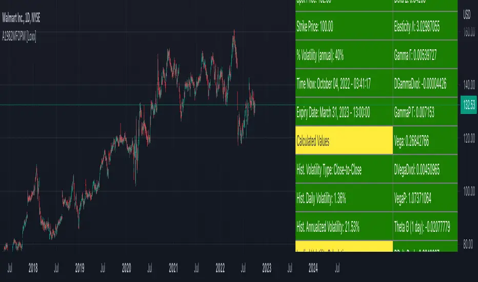
Black-76 Options on Futures [Loxx]Black-76 Options on Futures is an adaptation of the Black-Scholes-Merton Option Pricing Model including Analytical Greeks and implied volatility calculations. The following information is an excerpt from Espen Gaarder Haug's book "Option Pricing Formulas". This version is to price Options on Futures. The options sensitivities (Greeks) are the partial derivatives of the Black-Scholes-Merton ( BSM ) formula. Analytical Greeks for our purposes here are broken down into various categories:
Delta Greeks: Delta, DDeltaDvol, Elasticity
Gamma Greeks: Gamma, GammaP, DGammaDvol, Speed
Vega Greeks: Vega , DVegaDvol/Vomma, VegaP
Theta Greeks: Theta
Rate/Carry Greeks: Rho futures option
Probability Greeks: StrikeDelta, Risk Neutral Density
(See the code for more details)
Black-Scholes-Merton Option Pricing
The Black-Scholes-Merton model can be "generalized" by incorporating a cost-of-carry rate b. This model can be used to price European options on stocks, stocks paying a continuous dividend yield, options on futures , and currency options:
c = S * e^((b - r) * T) * N(d1) - X * e^(-r * T) * N(d2)
p = X * e^(-r * T) * N(-d2) - S * e^((b - r) * T) * N(-d1)
where
d1 = (log(S / X) + (b + v^2 / 2) * T) / (v * T^0.5)
d2 = d1 - v * T^0.5
b = r ... gives the Black and Scholes (1973) stock option model.
b = r — q ... gives the Merton (1973) stock option model with continuous dividend yield q.
b = 0 ... gives the Black (1976) futures option model. <== this is the one used for this indicator!
b = 0 and r = 0 ... gives the Asay (1982) margined futures option model.
b = r — rf ... gives the Garman and Kohlhagen (1983) currency option model.
Inputs
S = Stock price.
X = Strike price of option.
T = Time to expiration in years.
r = Risk-free rate
d = dividend yield
v = Volatility of the underlying asset price
cnd (x) = The cumulative normal distribution function
nd(x) = The standard normal density function
convertingToCCRate(r, cmp ) = Rate compounder
gImpliedVolatilityNR(string CallPutFlag, float S, float x, float T, float r, float b, float cm , float epsilon) = Implied volatility via Newton Raphson
gBlackScholesImpVolBisection(string CallPutFlag, float S, float x, float T, float r, float b, float cm ) = implied volatility via bisection
Implied Volatility: The Bisection Method
The Newton-Raphson method requires knowledge of the partial derivative of the option pricing formula with respect to volatility ( vega ) when searching for the implied volatility . For some options (exotic and American options in particular), vega is not known analytically. The bisection method is an even simpler method to estimate implied volatility when vega is unknown. The bisection method requires two initial volatility estimates (seed values):
1. A "low" estimate of the implied volatility , al, corresponding to an option value, CL
2. A "high" volatility estimate, aH, corresponding to an option value, CH
The option market price, Cm , lies between CL and cH . The bisection estimate is given as the linear interpolation between the two estimates:
v(i + 1) = v(L) + (c(m) - c(L)) * (v(H) - v(L)) / (c(H) - c(L))
Replace v(L) with v(i + 1) if c(v(i + 1)) < c(m), or else replace v(H) with v(i + 1) if c(v(i + 1)) > c(m) until |c(m) - c(v(i + 1))| <= E, at which point v(i + 1) is the implied volatility and E is the desired degree of accuracy.
Implied Volatility: Newton-Raphson Method
The Newton-Raphson method is an efficient way to find the implied volatility of an option contract. It is nothing more than a simple iteration technique for solving one-dimensional nonlinear equations (any introductory textbook in calculus will offer an intuitive explanation). The method seldom uses more than two to three iterations before it converges to the implied volatility . Let
v(i + 1) = v(i) + (c(v(i)) - c(m)) / (dc / dv (i))
until |c(m) - c(v(i + 1))| <= E at which point v(i + 1) is the implied volatility , E is the desired degree of accuracy, c(m) is the market price of the option, and dc/ dv (i) is the vega of the option evaluaated at v(i) (the sensitivity of the option value for a small change in volatility ).
Things to know
Only works on the daily timeframe and for the current source price.
You can adjust the text size to fit the screen
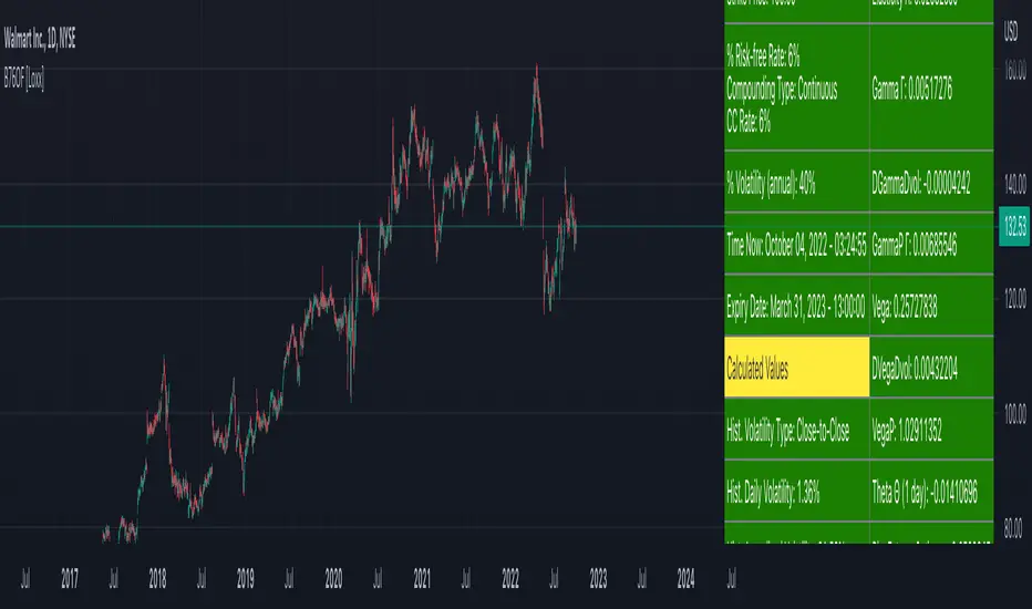
Garman and Kohlhagen (1983) for Currency Options [Loxx]Garman and Kohlhagen (1983) for Currency Options is an adaptation of the Black-Scholes-Merton Option Pricing Model including Analytical Greeks and implied volatility calculations. The following information is an excerpt from Espen Gaarder Haug's book "Option Pricing Formulas". This version of BSMOPM is to price Currency Options. The options sensitivities (Greeks) are the partial derivatives of the Black-Scholes-Merton ( BSM ) formula. Analytical Greeks for our purposes here are broken down into various categories:
Delta Greeks: Delta, DDeltaDvol, Elasticity
Gamma Greeks: Gamma, GammaP, DGammaDSpot/speed, DGammaDvol/Zomma
Vega Greeks: Vega , DVegaDvol/Vomma, VegaP, Speed
Theta Greeks: Theta
Rate/Carry Greeks: Rho, Rho futures option, Carry Rho, Phi/Rho2
Probability Greeks: StrikeDelta, Risk Neutral Density
(See the code for more details)
Black-Scholes-Merton Option Pricing for Currency Options
The Garman and Kohlhagen (1983) modified Black-Scholes model can be used to price European currency options; see also Grabbe (1983). The model is mathematically equivalent to the Merton (1973) model presented earlier. The only difference is that the dividend yield is replaced by the risk-free rate of the foreign currency rf:
c = S * e^(-rf * T) * N(d1) - X * e^(-r * T) * N(d2)
p = X * e^(-r * T) * N(-d2) - S * e^(-rf * T) * N(-d1)
where
d1 = (log(S / X) + (r - rf + v^2 / 2) * T) / (v * T^0.5)
d2 = d1 - v * T^0.5
For more information on currency options, see DeRosa (2000)
Inputs
S = Stock price.
X = Strike price of option.
T = Time to expiration in years.
r = Risk-free rate
rf = Risk-free rate of the foreign currency
v = Volatility of the underlying asset price
cnd (x) = The cumulative normal distribution function
nd(x) = The standard normal density function
convertingToCCRate(r, cmp ) = Rate compounder
gImpliedVolatilityNR(string CallPutFlag, float S, float x, float T, float r, float b, float cm , float epsilon) = Implied volatility via Newton Raphson
gBlackScholesImpVolBisection(string CallPutFlag, float S, float x, float T, float r, float b, float cm ) = implied volatility via bisection
Implied Volatility: The Bisection Method
The Newton-Raphson method requires knowledge of the partial derivative of the option pricing formula with respect to volatility ( vega ) when searching for the implied volatility . For some options (exotic and American options in particular), vega is not known analytically. The bisection method is an even simpler method to estimate implied volatility when vega is unknown. The bisection method requires two initial volatility estimates (seed values):
1. A "low" estimate of the implied volatility , al, corresponding to an option value, CL
2. A "high" volatility estimate, aH, corresponding to an option value, CH
The option market price, Cm , lies between CL and cH . The bisection estimate is given as the linear interpolation between the two estimates:
v(i + 1) = v(L) + (c(m) - c(L)) * (v(H) - v(L)) / (c(H) - c(L))
Replace v(L) with v(i + 1) if c(v(i + 1)) < c(m), or else replace v(H) with v(i + 1) if c(v(i + 1)) > c(m) until |c(m) - c(v(i + 1))| <= E, at which point v(i + 1) is the implied volatility and E is the desired degree of accuracy.
Implied Volatility: Newton-Raphson Method
The Newton-Raphson method is an efficient way to find the implied volatility of an option contract. It is nothing more than a simple iteration technique for solving one-dimensional nonlinear equations (any introductory textbook in calculus will offer an intuitive explanation). The method seldom uses more than two to three iterations before it converges to the implied volatility . Let
v(i + 1) = v(i) + (c(v(i)) - c(m)) / (dc / dv (i))
until |c(m) - c(v(i + 1))| <= E at which point v(i + 1) is the implied volatility , E is the desired degree of accuracy, c(m) is the market price of the option, and dc/ dv (i) is the vega of the option evaluaated at v(i) (the sensitivity of the option value for a small change in volatility ).
Things to know
Only works on the daily timeframe and for the current source price.
You can adjust the text size to fit the screen
Related indicators:
BSM OPM 1973 w/ Continuous Dividend Yield
Black-Scholes 1973 OPM on Non-Dividend Paying Stocks
Generalized Black-Scholes-Merton w/ Analytical Greeks
Generalized Black-Scholes-Merton Option Pricing Formula
Sprenkle 1964 Option Pricing Model w/ Num. Greeks
Modified Bachelier Option Pricing Model w/ Num. Greeks
Bachelier 1900 Option Pricing Model w/ Numerical Greeks

BSM OPM 1973 w/ Continuous Dividend Yield [Loxx]Generalized Black-Scholes-Merton w/ Analytical Greeks is an adaptation of the Black-Scholes-Merton Option Pricing Model including Analytical Greeks and implied volatility calculations. The following information is an excerpt from Espen Gaarder Haug's book "Option Pricing Formulas". The options sensitivities (Greeks) are the partial derivatives of the Black-Scholes-Merton ( BSM ) formula. Analytical Greeks for our purposes here are broken down into various categories:
Delta Greeks: Delta, DDeltaDvol, Elasticity
Gamma Greeks: Gamma, GammaP, DGammaDSpot/speed, DGammaDvol/Zomma
Vega Greeks: Vega , DVegaDvol/Vomma, VegaP
Theta Greeks: Theta
Rate/Carry Greeks: Rho, Rho futures option, Carry Rho, Phi/Rho2
Probability Greeks: StrikeDelta, Risk Neutral Density
(See the code for more details)
Black-Scholes-Merton Option Pricing
The Black-Scholes-Merton model can be "generalized" by incorporating a cost-of-carry rate b. This model can be used to price European options on stocks, stocks paying a continuous dividend yield, options on futures, and currency options:
c = S * e^((b - r) * T) * N(d1) - X * e^(-r * T) * N(d2)
p = X * e^(-r * T) * N(-d2) - S * e^((b - r) * T) * N(-d1)
where
d1 = (log(S / X) + (b + v^2 / 2) * T) / (v * T^0.5)
d2 = d1 - v * T^0.5
b = r ... gives the Black and Scholes (1973) stock option model.
b = r — q ... gives the Merton (1973) stock option model with continuous dividend yield q. <== this is the one used for this indicator!
b = 0 ... gives the Black (1976) futures option model.
b = 0 and r = 0 ... gives the Asay (1982) margined futures option model.
b = r — rf ... gives the Garman and Kohlhagen (1983) currency option model.
Inputs
S = Stock price.
X = Strike price of option.
T = Time to expiration in years.
r = Risk-free rate
d = dividend yield
v = Volatility of the underlying asset price
cnd (x) = The cumulative normal distribution function
nd(x) = The standard normal density function
convertingToCCRate(r, cmp ) = Rate compounder
gImpliedVolatilityNR(string CallPutFlag, float S, float x, float T, float r, float b, float cm , float epsilon) = Implied volatility via Newton Raphson
gBlackScholesImpVolBisection(string CallPutFlag, float S, float x, float T, float r, float b, float cm ) = implied volatility via bisection
Implied Volatility: The Bisection Method
The Newton-Raphson method requires knowledge of the partial derivative of the option pricing formula with respect to volatility ( vega ) when searching for the implied volatility . For some options (exotic and American options in particular), vega is not known analytically. The bisection method is an even simpler method to estimate implied volatility when vega is unknown. The bisection method requires two initial volatility estimates (seed values):
1. A "low" estimate of the implied volatility , al, corresponding to an option value, CL
2. A "high" volatility estimate, aH, corresponding to an option value, CH
The option market price, Cm , lies between CL and cH . The bisection estimate is given as the linear interpolation between the two estimates:
v(i + 1) = v(L) + (c(m) - c(L)) * (v(H) - v(L)) / (c(H) - c(L))
Replace v(L) with v(i + 1) if c(v(i + 1)) < c(m), or else replace v(H) with v(i + 1) if c(v(i + 1)) > c(m) until |c(m) - c(v(i + 1))| <= E, at which point v(i + 1) is the implied volatility and E is the desired degree of accuracy.
Implied Volatility: Newton-Raphson Method
The Newton-Raphson method is an efficient way to find the implied volatility of an option contract. It is nothing more than a simple iteration technique for solving one-dimensional nonlinear equations (any introductory textbook in calculus will offer an intuitive explanation). The method seldom uses more than two to three iterations before it converges to the implied volatility . Let
v(i + 1) = v(i) + (c(v(i)) - c(m)) / (dc / dv (i))
until |c(m) - c(v(i + 1))| <= E at which point v(i + 1) is the implied volatility , E is the desired degree of accuracy, c(m) is the market price of the option, and dc/ dv (i) is the vega of the option evaluaated at v(i) (the sensitivity of the option value for a small change in volatility ).
Things to know
Only works on the daily timeframe and for the current source price.
You can adjust the text size to fit the screen

Black-Scholes 1973 OPM on Non-Dividend Paying Stocks [Loxx]Black-Scholes 1973 OPM on Non-Dividend Paying Stocks is an adaptation of the Black-Scholes-Merton Option Pricing Model including Analytical Greeks and implied volatility calculations. Making b equal to r yields the BSM model where dividends are not considered. The following information is an excerpt from Espen Gaarder Haug's book "Option Pricing Formulas". The options sensitivities (Greeks) are the partial derivatives of the Black-Scholes-Merton ( BSM ) formula. For our purposes here are, Analytical Greeks are broken down into various categories:
Delta Greeks: Delta, DDeltaDvol, Elasticity
Gamma Greeks: Gamma, GammaP, DGammaDSpot/speed, DGammaDvol/Zomma
Vega Greeks: Vega , DVegaDvol/Vomma, VegaP
Theta Greeks: Theta
Rate/Carry Greeks: Rho
Probability Greeks: StrikeDelta, Risk Neutral Density
(See the code for more details)
Black-Scholes-Merton Option Pricing
The BSM formula and its binomial counterpart may easily be the most used "probability model/tool" in everyday use — even if we con- sider all other scientific disciplines. Literally tens of thousands of people, including traders, market makers, and salespeople, use option formulas several times a day. Hardly any other area has seen such dramatic growth as the options and derivatives businesses. In this chapter we look at the various versions of the basic option formula. In 1997 Myron Scholes and Robert Merton were awarded the Nobel Prize (The Bank of Sweden Prize in Economic Sciences in Memory of Alfred Nobel). Unfortunately, Fischer Black died of cancer in 1995 before he also would have received the prize.
It is worth mentioning that it was not the option formula itself that Myron Scholes and Robert Merton were awarded the Nobel Prize for, the formula was actually already invented, but rather for the way they derived it — the replicating portfolio argument, continuous- time dynamic delta hedging, as well as making the formula consistent with the capital asset pricing model (CAPM). The continuous dynamic replication argument is unfortunately far from robust. The popularity among traders for using option formulas heavily relies on hedging options with options and on the top of this dynamic delta hedging, see Higgins (1902), Nelson (1904), Mello and Neuhaus (1998), Derman and Taleb (2005), as well as Haug (2006) for more details on this topic. In any case, this book is about option formulas and not so much about how to derive them.
Provided here are the various versions of the Black-Scholes-Merton formula presented in the literature. All formulas in this section are originally derived based on the underlying asset S follows a geometric Brownian motion
dS = mu * S * dt + v * S * dz
where t is the expected instantaneous rate of return on the underlying asset, a is the instantaneous volatility of the rate of return, and dz is a Wiener process.
The formula derived by Black and Scholes (1973) can be used to value a European option on a stock that does not pay dividends before the option's expiration date. Letting c and p denote the price of European call and put options, respectively, the formula states that
c = S * N(d1) - X * e^(-r * T) * N(d2)
p = X * e^(-r * T) * N(d2) - S * N(d1)
where
d1 = (log(S / X) + (r + v^2 / 2) * T) / (v * T^0.5)
d2 = (log(S / X) + (r - v^2 / 2) * T) / (v * T^0.5) = d1 - v * T^0.5
**This version of the Black-Scholes formula can also be used to price American call options on a non-dividend-paying stock, since it will never be optimal to exercise the option before expiration.**
Inputs
S = Stock price.
X = Strike price of option.
T = Time to expiration in years.
r = Risk-free rate
b = Cost of carry
v = Volatility of the underlying asset price
cnd (x) = The cumulative normal distribution function
nd(x) = The standard normal density function
convertingToCCRate(r, cmp ) = Rate compounder
gImpliedVolatilityNR(string CallPutFlag, float S, float x, float T, float r, float b, float cm , float epsilon) = Implied volatility via Newton Raphson
gBlackScholesImpVolBisection(string CallPutFlag, float S, float x, float T, float r, float b, float cm ) = implied volatility via bisection
Implied Volatility: The Bisection Method
The Newton-Raphson method requires knowledge of the partial derivative of the option pricing formula with respect to volatility ( vega ) when searching for the implied volatility . For some options (exotic and American options in particular), vega is not known analytically. The bisection method is an even simpler method to estimate implied volatility when vega is unknown. The bisection method requires two initial volatility estimates (seed values):
1. A "low" estimate of the implied volatility , al, corresponding to an option value, CL
2. A "high" volatility estimate, aH, corresponding to an option value, CH
The option market price, Cm , lies between CL and cH . The bisection estimate is given as the linear interpolation between the two estimates:
v(i + 1) = v(L) + (c(m) - c(L)) * (v(H) - v(L)) / (c(H) - c(L))
Replace v(L) with v(i + 1) if c(v(i + 1)) < c(m), or else replace v(H) with v(i + 1) if c(v(i + 1)) > c(m) until |c(m) - c(v(i + 1))| <= E, at which point v(i + 1) is the implied volatility and E is the desired degree of accuracy.
Implied Volatility: Newton-Raphson Method
The Newton-Raphson method is an efficient way to find the implied volatility of an option contract. It is nothing more than a simple iteration technique for solving one-dimensional nonlinear equations (any introductory textbook in calculus will offer an intuitive explanation). The method seldom uses more than two to three iterations before it converges to the implied volatility . Let
v(i + 1) = v(i) + (c(v(i)) - c(m)) / (dc / dv (i))
until |c(m) - c(v(i + 1))| <= E at which point v(i + 1) is the implied volatility , E is the desired degree of accuracy, c(m) is the market price of the option, and dc/ dv (i) is the vega of the option evaluaated at v(i) (the sensitivity of the option value for a small change in volatility ).
Things to know
Only works on the daily timeframe and for the current source price.
You can adjust the text size to fit the screen

Generalized Black-Scholes-Merton w/ Analytical Greeks [Loxx]Generalized Black-Scholes-Merton w/ Analytical Greeks is an adaptation of the Black-Scholes-Merton Option Pricing Model including Analytical Greeks and implied volatility calculations. The following information is an excerpt from Espen Gaarder Haug's book "Option Pricing Formulas". The options sensitivities (Greeks) are the partial derivatives of the Black-Scholes-Merton (BSM) formula. Analytical Greeks for our purposes here are broken down into various categories:
Delta Greeks: Delta, DDeltaDvol, Elasticity
Gamma Greeks: Gamma, GammaP, DGammaDSpot/speed, DGammaDvol/Zomma
Vega Greeks: Vega, DVegaDvol/Vomma, VegaP
Theta Greeks: Theta
Rate/Carry Greeks: Rho, Rho futures option, Carry Rho, Phi/Rho2
Probability Greeks: StrikeDelta, Risk Neutral Density
(See the code for more details)
Black-Scholes-Merton Option Pricing
The BSM formula and its binomial counterpart may easily be the most used "probability model/tool" in everyday use — even if we con- sider all other scientific disciplines. Literally tens of thousands of people, including traders, market makers, and salespeople, use option formulas several times a day. Hardly any other area has seen such dramatic growth as the options and derivatives businesses. In this chapter we look at the various versions of the basic option formula. In 1997 Myron Scholes and Robert Merton were awarded the Nobel Prize (The Bank of Sweden Prize in Economic Sciences in Memory of Alfred Nobel). Unfortunately, Fischer Black died of cancer in 1995 before he also would have received the prize.
It is worth mentioning that it was not the option formula itself that Myron Scholes and Robert Merton were awarded the Nobel Prize for, the formula was actually already invented, but rather for the way they derived it — the replicating portfolio argument, continuous- time dynamic delta hedging, as well as making the formula consistent with the capital asset pricing model (CAPM). The continuous dynamic replication argument is unfortunately far from robust. The popularity among traders for using option formulas heavily relies on hedging options with options and on the top of this dynamic delta hedging, see Higgins (1902), Nelson (1904), Mello and Neuhaus (1998), Derman and Taleb (2005), as well as Haug (2006) for more details on this topic. In any case, this book is about option formulas and not so much about how to derive them.
Provided here are the various versions of the Black-Scholes-Merton formula presented in the literature. All formulas in this section are originally derived based on the underlying asset S follows a geometric Brownian motion
dS = mu * S * dt + v * S * dz
where t is the expected instantaneous rate of return on the underlying asset, a is the instantaneous volatility of the rate of return, and dz is a Wiener process.
The formula derived by Black and Scholes (1973) can be used to value a European option on a stock that does not pay dividends before the option's expiration date. Letting c and p denote the price of European call and put options, respectively, the formula states that
c = S * N(d1) - X * e^(-r * T) * N(d2)
p = X * e^(-r * T) * N(d2) - S * N(d1)
where
d1 = (log(S / X) + (r + v^2 / 2) * T) / (v * T^0.5)
d2 = (log(S / X) + (r - v^2 / 2) * T) / (v * T^0.5) = d1 - v * T^0.5
Inputs
S = Stock price.
X = Strike price of option.
T = Time to expiration in years.
r = Risk-free rate
b = Cost of carry
v = Volatility of the underlying asset price
cnd (x) = The cumulative normal distribution function
nd(x) = The standard normal density function
convertingToCCRate(r, cmp ) = Rate compounder
gImpliedVolatilityNR(string CallPutFlag, float S, float x, float T, float r, float b, float cm , float epsilon) = Implied volatility via Newton Raphson
gBlackScholesImpVolBisection(string CallPutFlag, float S, float x, float T, float r, float b, float cm ) = implied volatility via bisection
Implied Volatility: The Bisection Method
The Newton-Raphson method requires knowledge of the partial derivative of the option pricing formula with respect to volatility ( vega ) when searching for the implied volatility . For some options (exotic and American options in particular), vega is not known analytically. The bisection method is an even simpler method to estimate implied volatility when vega is unknown. The bisection method requires two initial volatility estimates (seed values):
1. A "low" estimate of the implied volatility , al, corresponding to an option value, CL
2. A "high" volatility estimate, aH, corresponding to an option value, CH
The option market price, Cm , lies between CL and cH . The bisection estimate is given as the linear interpolation between the two estimates:
v(i + 1) = v(L) + (c(m) - c(L)) * (v(H) - v(L)) / (c(H) - c(L))
Replace v(L) with v(i + 1) if c(v(i + 1)) < c(m), or else replace v(H) with v(i + 1) if c(v(i + 1)) > c(m) until |c(m) - c(v(i + 1))| <= E, at which point v(i + 1) is the implied volatility and E is the desired degree of accuracy.
Implied Volatility: Newton-Raphson Method
The Newton-Raphson method is an efficient way to find the implied volatility of an option contract. It is nothing more than a simple iteration technique for solving one-dimensional nonlinear equations (any introductory textbook in calculus will offer an intuitive explanation). The method seldom uses more than two to three iterations before it converges to the implied volatility . Let
v(i + 1) = v(i) + (c(v(i)) - c(m)) / (dc / dv (i))
until |c(m) - c(v(i + 1))| <= E at which point v(i + 1) is the implied volatility , E is the desired degree of accuracy, c(m) is the market price of the option, and dc/ dv (i) is the vega of the option evaluaated at v(i) (the sensitivity of the option value for a small change in volatility ).
Things to know
Only works on the daily timeframe and for the current source price.
You can adjust the text size to fit the screen

StapleIndicatorsLibrary "StapleIndicators"
This Library provides some common indicators commonly referenced from other studies in Pine Script
squeeze(bbSrc, bbPeriod, bbDev, kcSrc, kcPeriod, kcATR, signalPeriod) Volatility Squeeze
Parameters:
bbSrc : (Optional) Bollinger Bands Source. By default close
bbPeriod : (Optional) Bollinger Bands Period. By default 20
bbDev : (Optional) Bollinger Bands Standard Deviation. By default 2.0
kcSrc : (Optional) Keltner Channel Source. By default close
kcPeriod : (Optional) Keltner Channel Period. By default 20
kcATR : (Optional) Keltner Channel ATR Multiplier. By default 1.5
signalPeriod : (Optional) Keltner Channel ATR Multiplier. By default 1.5
Returns:
adx(diPeriod, adxPeriod, signalPeriod, adxTier1, adxTier2, adxTier3) ADX: Average Directional Index
Parameters:
diPeriod : (Optional) Directional Indicator Period. By default 14
adxPeriod : (Optional) ADX Smoothing. By default 14
signalPeriod : (Optional) Signal Period. By default 13
adxTier1 : (Optional) ADX Tier #1 Level. By default 20
adxTier2 : (Optional) ADX Tier #2 Level. By default 15
adxTier3 : (Optional) ADX Tier #3 Level. By default 10
Returns:
smaPreset(srcMa) Delivers a set of frequently used Simple Moving Averages
Parameters:
srcMa : (Optional) MA Source. By default 'close'
Returns:
emaPreset(srcMa) Delivers a set of frequently used Exponential Moving Averages
Parameters:
srcMa : (Optional) MA Source. By default 'close'
Returns:
maSelect(ma, srcMa) Filters and outputs the selected MA
Parameters:
ma : (Optional) MA text. By default 'Ema-21'
srcMa : (Optional) MA Source. By default 'close'
Returns: maSelected
periodAdapt(modeAdaptative, src, maxLen, minLen) Adaptative Period
Parameters:
modeAdaptative : (Optional) Adaptative Mode. By default 'Average'
src : (Optional) Source. By default 'close'
maxLen : (Optional) Max Period. By default '60'
minLen : (Optional) Min Period. By default '4'
Returns: periodAdaptative
azlema(modeAdaptative, srcMa) Azlema: Adaptative Zero-Lag Ema
Parameters:
modeAdaptative : (Optional) Adaptative Mode. By default 'Average'
srcMa : (Optional) MA Source. By default 'close'
Returns: azlema
ssma(lsmaVar, srcMa, periodMa) SSMA: Smooth Simple MA
Parameters:
lsmaVar : Linear Regression Curve.
srcMa : (Optional) MA Source. By default 'close'
periodMa : (Optional) MA Period. By default '13'
Returns: ssma
jvf(srcMa, periodMa) Jurik Volatility Factor
Parameters:
srcMa : (Optional) MA Source. By default 'close'
periodMa : (Optional) MA Period. By default '7'
Returns:
jBands(srcMa, periodMa) Jurik Bands
Parameters:
srcMa : (Optional) MA Source. By default 'close'
periodMa : (Optional) MA Period. By default '7'
Returns:
jma(srcMa, periodMa, phase) Jurik MA (JMA)
Parameters:
srcMa : (Optional) MA Source. By default 'close'
periodMa : (Optional) MA Period. By default '7'
phase : (Optional) Phase. By default '50'
Returns: jma
maCustom(ma, srcMa, periodMa, lrOffset, almaOffset, almaSigma, jmaPhase, azlemaMode) Creates a custom Moving Average
Parameters:
ma : (Optional) MA text. By default 'Ema'
srcMa : (Optional) MA Source. By default 'close'
periodMa : (Optional) MA Period. By default '13'
lrOffset : (Optional) Linear Regression Offset. By default '0'
almaOffset : (Optional) Alma Offset. By default '0.85'
almaSigma : (Optional) Alma Sigma. By default '6'
jmaPhase : (Optional) JMA Phase. By default '50'
azlemaMode : (Optional) Azlema Adaptative Mode. By default 'Average'
Returns: maTF
