Tight Range Display with Background🌟 Tight Range Transparency Display with Background
What Is This Indicator?
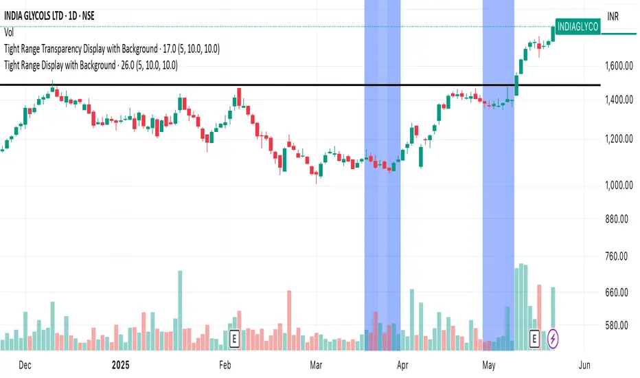
Hey traders! Ever wanted a simple way to spot those quiet, low-volatility moments in the market that often signal a big move is coming? The Tight Range Transparency Display with Background does exactly that! This indicator highlights periods where the price is moving in a tight range—think of it as the calm before the storm. It paints the chart background blue to show these zones, with the shade getting darker the tighter the range becomes. It’s like having a visual cue to say, “Hey, something might be brewing here!”
Why You’ll Love It
Spot Key Moments Easily: The blue background makes it super easy to see when the market is in a tight range, which often happens before breakouts or big trends.
Customizable Settings: You can tweak the range thresholds to match your trading style—whether you’re looking for super tight zones or slightly broader ones.
Visual Clarity: The background gets darker when the range is tighter, giving you a quick sense of how compressed the price action is.
Perfect for Any Market: Works on stocks, forex, crypto, or any chart you trade, across any timeframe.
How to Use It
Add It to Your Chart:
Just copy this script into TradingView’s Pine Editor and hit "Add to Chart." It’ll overlay right on your price chart.
Tweak the Settings:
Open the indicator settings and use the dropdown menus to pick your preferred "Tight Range %" and "Wide Range %." For example, set a Tight Range % of 2.0% to catch smaller ranges, or go higher like 10.0% for broader ones.
You can also adjust the ATR Period (default is 5) to make the indicator more or less sensitive to recent price swings.
Watch for the Blue Background:
When the price enters a tight range, the chart background turns blue. The darker the blue, the tighter the range—meaning a potential breakout could be closer!
Trade Smarter:
Use these tight range zones to prepare for potential breakouts. For example, if you see a dark blue background, it might be a good time to watch for a big price move.
Pair this with other tools like support/resistance levels or volume spikes to confirm your trades.
Who Is This For?
Swing Traders: Perfect for spotting consolidation zones before a big swing.
Breakout Traders: Tight ranges often lead to breakouts—use this to time your entries.
Smart Money Followers: If you’re into smart money concepts, tight ranges can signal accumulation or distribution phases.
Beginners & Pros Alike: It’s easy to use for new traders but powerful enough for seasoned pros.
Real-World Example
Imagine you’re trading a stock on a 1-hour chart. You notice the background turns blue, and it’s getting darker over a few bars. This tells you the price range is tightening—maybe the stock is consolidating after a big move. You check your other indicators, see a volume spike, and spot a breakout above resistance. Boom! You catch the next big trend, all because this indicator helped you focus on the right moment.
Tips for Best Results
Try Different Timeframes: Tight ranges on a 15-minute chart might signal short-term moves, while a daily chart could highlight bigger trends.
Adjust for Your Market: For volatile markets like crypto, you might want a higher Tight Range % (e.g., 10.0%). For calmer markets like forex, try a lower setting (e.g., 2.0%).
Combine with Other Tools: Use this alongside trendlines, moving averages, or volume indicators to confirm your setups.
Why I Made This
I created this indicator because I wanted a simple, visual way to spot those critical low-volatility zones without cluttering my chart. The dynamic background color makes it intuitive to see when the market is “coiling up” for a potential move. I hope it helps you find better trading opportunities just like it does for me!
Let’s Connect
If you find this indicator helpful, I’d love to hear about it! Drop a comment or a rating to let me know how it’s working for you. Got ideas to make it even better? Feel free to message me on TradingView—I’m always open to suggestions.
Published On
Date: May 22, 2025
Happy trading, and may your charts always be in your favor! 🚀
How to Publish on TradingView
Open Pine Editor:
On TradingView, open a chart and go to the Pine Editor tab at the bottom.
Paste the Code:
Copy the script you provided and paste it into the Pine Editor.
Compile:
Click "Add to Chart" to ensure it compiles without errors.
Publish:
Click the "Publish Script" button (paper plane icon) in the Pine Editor.
Select "Publish New Script."
Add the Description:
Title: "Tight Range Transparency Display with Background"
Description: Copy the content above into the description field.
Visibility: Choose "Public" to share with everyone (or "Invite-Only" for restricted access).
Tags: Add tags like "tight range", "breakout", "smart money", "volatility", "swing trading".
Screenshot: Add a screenshot of the indicator on a chart, showing the blue background during a tight range.
Submit:
Click "Publish" to submit. TradingView will review it and make it live if it meets their guidelines.
Additional Notes
Screenshot Tip: Use a chart where the blue background is clearly visible (e.g., during a consolidation period) to make the indicator’s effect stand out.
Engage with Users: After publishing, respond to comments and feedback to build a positive reputation on TradingView.
This content is designed to be approachable and engaging, helping traders understand the value of your indicator and encouraging them to try it out.
חפש סקריפטים עבור "tradingview界面调整"
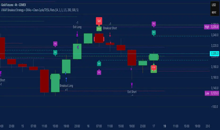
VWAP Breakout Strategy + EMAs + Clean Cycle/TP/SL PlotsHere’s a quick user-guide to get you up and running with your “VWAP Breakout Strategy + EMAs + Clean Cycle/TP/SL Plots” script in TradingView:
⸻
1. Installing the Script
1. Open TradingView, go to Pine Editor (bottom panel).
2. Paste in your full Pine-v6 code and hit Add to chart.
3. Save it (“Save as…”): give it a memorable name (e.g. “VWAP Breakout+EMAs”).
⸻
2. Configuring Your Inputs
Once it’s on the chart, click the ⚙️ Settings icon to tune:
Setting Default What it does
ATR Length 14 Period for average true range (volatility measure)
ATR Multiplier for Stop 1.5 How many ATRs away your stop-loss sits
TP1 / TP2 Multipliers (ATR) 1.0 / 2.0 Distance of TP1 and TP2 in ATR multiples
Show VWAP / EMAs On Toggles the blue VWAP line & EMAs (100/34/5)
Full Cycle Range Points 200 Height of the shaded “cycle zone”
Pivot Lookback 5 How many bars back to detect a pivot low
Round Number Step 500 Spacing of your dotted horizontal lines
Show TP/SL Labels On Toggles all the “ENTRY”, “TP1”, “TP2”, “STOP” tags
Feel free to adjust ATR multipliers and cycle-zone size based on the instrument’s typical range.
⸻
3. Reading the Signals
• Long Entry:
• Trigger: price crosses above VWAP
• You’ll see a green “Buy” tag at the low of the signal bar, plus an “ENTRY (Long)” label at the close.
• Stop is plotted as a red dashed line below (ATR × 1.5), and TP1/TP2 as teal and purple lines above.
• Short Entry:
• Trigger: price crosses below VWAP
• A red “Sell” tag appears at the high, with “ENTRY (Short)” at the close.
• Stop is the green line above; TP1/TP2 are dashed teal/purple lines below.
⸻
4. Full Cycle Zone
Whenever a new pivot low is detected (using your Pivot Lookback), the script deletes the old box and draws a shaded yellow rectangle from that low up by “Full Cycle Range Points.”
• Use this to visualize the “maximum expected swing” from your pivot.
• You can quickly see whether price is still traveling within a normal cycle or has overstretched.
⸻
5. Round-Number Levels
With Show Round Number Levels enabled, you’ll always get horizontal dotted lines at the nearest multiples of your “Round Number Step” (e.g. every 500 points).
• These often act as psychological support/resistance.
• Handy to see confluence with VWAP or cycle-zone edges.
⸻
6. Tips & Best-Practices
• Timeframes: Apply on any intraday chart (5 min, 15 min, H1…), but match your ATR length & cycle-points to the timeframe’s typical range.
• Backtest first: Use the Strategy Tester tab to review performance, tweak ATR multipliers or cycle size, then optimize.
• Combine with context: Don’t trade VWAP breakouts blindly—look for confluence (e.g. support/resistance zones, higher-timeframe trend).
• Label clutter: If too many labels build up, you can toggle Show TP/SL Labels off and rely just on the lines.
⸻
That’s it! Once you’ve added it to your chart and dialed in the inputs, your entries, exits, cycle ranges, and key levels will all be plotted automatically. Feel free to experiment with the ATR multipliers and cycle-zone size until it fits your instrument’s personality. Happy trading!
Candle Height & Trend Probability DashboardDescription and Guide
Description:
This Pine Script for TradingView displays a dashboard that calculates the probability of price increases or decreases based on past price movements. It analyzes the last 30 candles (by default) and shows the probabilities for different timeframes (from 1 minute to 1 week). Additionally, it checks volatility using the ATR indicator.
Script Features:
Calculates probabilities of an upward (Up %) or downward (Down %) price move based on past candles.
Displays a dashboard showing probabilities for multiple timeframes.
Color-coded probability display:
Green if the upward probability exceeds a set threshold.
Red if the downward probability exceeds the threshold.
Yellow if neither threshold is exceeded.
Considers volatility using the ATR indicator.
Triggers alerts when probabilities exceed specific values.
How to Use:
Insert the script into TradingView: Copy and paste the script into the Pine Script editor.
Adjust parameters:
lookback: Number of past candles used for calculation (default: 30).
alertThresholdUp & alertThresholdDown: Thresholds for probabilities (default: 51%).
volatilityLength & volatilityThreshold: ATR volatility settings.
dashboardPosition: Choose where the dashboard appears on the chart.
Enable visualization: The dashboard will be displayed over the chart.
Set alerts: The script triggers notifications when probabilities exceed set thresholds.

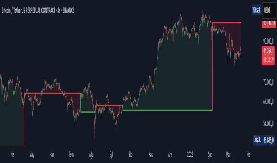
Dynamic Support and Resistance ### Indicator: Dynamic Support and Resistance
#### Overview:
The *Dynamic Support and Resistance* indicator is a powerful tool designed to help traders identify key price levels on a chart. It dynamically calculates support and resistance levels based on pivot points and the Average True Range (ATR). The indicator also highlights broken support and resistance zones, providing visual cues for potential trend reversals or continuations.
---
### Key Features:
1. *Dynamic Support and Resistance Levels*:
- The indicator identifies support and resistance levels using pivot highs and lows within a user-defined range.
- These levels are adjusted using the ATR to account for market volatility, making them more responsive to changing market conditions.
2. *Support and Resistance Zones*:
- The indicator draws boxes around the support and resistance levels, with customizable colors and widths.
- The width of the zones is determined by the ATR and a user-defined multiplier, allowing traders to adjust the sensitivity of the zones.
3. *Broken Zones*:
- When price breaks through a support or resistance zone, the zone is highlighted with a distinct color to indicate a potential shift in market sentiment.
- Traders can limit the number of broken zones displayed on the chart to avoid clutter.
4. *Customizable Inputs*:
- *Range Candle Count*: Defines the number of candles analyzed to determine pivot points. Increasing this value will result in fewer but more significant levels, while decreasing it will produce more levels that are sensitive to shorter-term price movements.
- *ATR Period*: Controls the sensitivity of the ATR calculation. A shorter period makes the ATR more responsive to recent price changes, while a longer period smooths it out.
- *Box Width Multiplier*: Adjusts the width of the support and resistance zones. A higher multiplier creates wider zones, which may be useful in more volatile markets.
- *Max Broken Zones*: Limits the number of broken zones displayed on the chart. This helps keep the chart clean and focused on the most recent breaks.
---
### How It Works:
1. *Pivot Points*:
- The indicator identifies pivot highs and lows within the specified range. These pivots serve as the basis for calculating support and resistance levels.
2. *ATR Adjustment*:
- The ATR is used to adjust the support and resistance levels, making them more dynamic and responsive to market volatility.
3. *Zone Creation*:
- Support and resistance zones are drawn as boxes around the pivot levels. The width of these zones is determined by the ATR and the box width multiplier.
4. *Zone Breaks*:
- When price breaks through a zone, the zone is highlighted with a distinct color, and the broken zone is added to an array. If the number of broken zones exceeds the user-defined limit, the oldest broken zone is removed from the chart.
---
### How to Use:
1. *Trend Identification*:
- Use the support and resistance levels to identify key price levels where the market may reverse or consolidate.
- Broken zones can signal potential trend reversals or continuations.
2. *Entry and Exit Points*:
- Traders can use the support and resistance zones as potential entry or exit points. For example, buying near support or selling near resistance.
- Broken zones can be used as confirmation for breakout strategies.
3. *Risk Management*:
- The width of the zones can help traders set stop-loss levels. For example, placing a stop-loss just outside a support or resistance zone.
4. *Customization*:
- Adjust the input parameters to suit your trading style and the specific market conditions. For example, increase the range candle count for longer-term analysis or decrease it for shorter-term trading.
---
### Who Should Use This Indicator?
- *Swing Traders*: Can use the indicator to identify key levels for potential reversals or breakouts.
- *Day Traders*: Can benefit from the dynamic levels and zones, especially in volatile markets.
- *Position Traders*: Can use the indicator to identify long-term support and resistance levels.
- *Breakout Traders*: Can use the broken zones to confirm breakouts and plan their trades accordingly.
---
### Input Parameters and Their Effects:
1. *Range Candle Count*:
- *Increase*: Produces fewer but more significant levels, suitable for longer-term analysis.
- *Decrease*: Produces more levels, sensitive to shorter-term price movements.
2. *ATR Period*:
- *Increase*: Smoothens the ATR, making the levels less sensitive to recent price changes.
- *Decrease*: Makes the ATR more responsive to recent price changes, resulting in more dynamic levels.
3. *Box Width Multiplier*:
- *Increase*: Creates wider zones, suitable for more volatile markets.
- *Decrease*: Creates narrower zones, suitable for less volatile markets.
4. *Max Broken Zones*:
- *Increase*: Displays more broken zones on the chart, providing more historical context.
- *Decrease*: Keeps the chart clean by displaying only the most recent broken zones.
---
### Conclusion:
The *Dynamic Support and Resistance* indicator is a versatile tool that can be adapted to various trading styles and market conditions. By dynamically adjusting to market volatility and highlighting key price levels, it provides traders with valuable insights into potential support and resistance areas. Whether you're a swing trader, day trader, or position trader, this indicator can help you make more informed trading decisions.
---
### Publishing on TradingView:
- *Title*: Dynamic Support and Resistance
- *Description*: A dynamic support and resistance indicator that uses pivot points and ATR to identify key price levels. Includes customizable support/resistance zones and highlights broken zones for breakout trading.
- *Tags*: support, resistance, ATR, pivot points, breakout, trading, indicator
- *Access*: Public or Invite-only, depending on your preference.
This indicator is ready to be published on TradingView, and the detailed description above will help users understand its functionality and how to use it effectively.

Trend Detection
#### *Description:*
This *Trend Detection* indicator is designed to help traders identify and confirm trends in the market using a combination of moving averages, volume analysis, and MACD filters. It provides clear visual signals for uptrends and downtrends, along with customizable settings to adapt to different trading styles and timeframes. The indicator is suitable for both beginners and advanced traders who want to improve their trend-following strategies.
---
#### *Key Features:*
1. *Trend Detection:*
- Uses *Moving Averages (MA)* to determine the overall trend direction.
- Supports multiple MA types: *SMA (Simple), **EMA (Exponential), **WMA (Weighted), and **HMA (Hull)*.
2. *Advanced Filters:*
- *MACD Filter:* Confirms trends using MACD crossovers.
- *Volume Filter:* Ensures trends are supported by above-average volume.
- *Multi-Timeframe Filter:* Validates trends using a higher timeframe (e.g., Daily or Weekly).
3. *Visual Signals:*
- Plots a *trend line* on the chart to indicate the current trend direction.
- Fills the background with *green* for uptrends and *red* for downtrends.
4. *Customizable Settings:*
- Adjust the *MA lengths, **MACD parameters, and **confirmation thresholds* to suit your trading strategy.
- Control the transparency of the background fill for better chart readability.
5. *Alerts:*
- Generates *buy/sell signals* when a trend is confirmed.
- Alerts can be set to trigger at the close of a candle for precise entry/exit points.
---
#### *How to Use:*
1. *Adding the Indicator:*
- Copy and paste the Pine Script code into the TradingView Pine Script editor.
- Add the indicator to your chart.
2. *Configuring the Settings:*
- *Trend Settings:*
- Choose the *MA type* (e.g., EMA for faster response, HMA for smoother trends).
- Set the *Trend MA Period* (e.g., 200 for long-term trends) and *Filter MA Period* (e.g., 100 for medium-term trends).
- *Advanced Filters:*
- Enable/disable the *MACD Filter* and adjust its parameters (Fast, Slow, Signal).
- Enable/disable the *Volume Filter* to ensure trends are supported by volume.
- *Multi-Timeframe Filter:*
- Enable this filter to validate trends using a higher timeframe (e.g., Daily or Weekly).
3. *Interpreting the Signals:*
- *Uptrend:* The trend line turns *green*, and the background is filled with a transparent green color.
- *Downtrend:* The trend line turns *red*, and the background is filled with a transparent red color.
- *Alerts:* Buy/sell signals are generated when the trend is confirmed.
4. *Using Alerts:*
- Set up alerts for *Buy Signal* (bullish reversal) and *Sell Signal* (bearish reversal).
- Alerts can be configured to trigger at the close of a candle for precise execution.
---
#### *Settings and Their Effects:*
1. *MA Type:*
- *SMA:* Smooth but lagging. Best for long-term trends.
- *EMA:* Faster response to price changes. Suitable for medium-term trends.
- *WMA:* Gives more weight to recent prices. Useful for short-term trends.
- *HMA:* Combines speed and smoothness. Ideal for all timeframes.
2. *Trend MA Period:*
- A longer period (e.g., 200) identifies long-term trends but may lag.
- A shorter period (e.g., 50) reacts faster but may produce false signals.
3. *Filter MA Period:*
- Acts as a secondary filter to confirm the trend.
- A shorter period (e.g., 50) provides tighter confirmation but may increase noise.
4. *MACD Filter:*
- Ensures trends are confirmed by MACD crossovers.
- Adjust the *Fast, **Slow, and **Signal* lengths to match your trading style.
5. *Volume Filter:*
- Ensures trends are supported by above-average volume.
- Reduces false signals during low-volume periods.
6. *Multi-Timeframe Filter:*
- Validates trends using a higher timeframe (e.g., Daily or Weekly).
- Increases reliability but may delay signals.
7. *Confirmation Value:*
- Sets the minimum percentage deviation from the trend MA required to confirm a trend.
- A higher value (e.g., 2.0%) reduces false signals but may delay trend detection.
8. *Confirmation Bars:*
- Sets the number of bars required to confirm a trend.
- A higher value (e.g., 5 bars) ensures sustained trends but may delay signals.
---
#### *Who Should Use This Indicator?*
1. *Trend Followers:*
- Traders who focus on identifying and riding long-term trends.
- Suitable for *swing traders* and *position traders*.
2. *Day Traders:*
- Can use shorter MA periods and faster filters (e.g., EMA, HMA) for intraday trends.
3. *Volume-Based Traders:*
- Traders who rely on volume confirmation to validate trends.
4. *Multi-Timeframe Traders:*
- Traders who use higher timeframes to confirm trends on lower timeframes.
5. *Beginners:*
- Easy-to-understand visual signals and alerts make it beginner-friendly.
6. *Advanced Traders:*
- Customizable settings allow for fine-tuning to match specific strategies.
---
#### *Example Use Cases:*
1. *Long-Term Investing:*
- Use a *200-period SMA* with a *Daily* higher timeframe filter to identify long-term trends.
- Enable the *Volume Filter* to ensure trends are supported by strong volume.
2. *Swing Trading:*
- Use a *50-period EMA* with a *4-hour* higher timeframe filter for medium-term trends.
- Enable the *MACD Filter* to confirm trend reversals.
3. *Day Trading:*
- Use a *20-period HMA* with a *1-hour* higher timeframe filter for short-term trends.
- Disable the *Volume Filter* for faster signals.
---
#### *Conclusion:*
The *Trend Detection* indicator is a versatile tool for traders of all levels. Its customizable settings and advanced filters make it suitable for various trading styles and timeframes. By combining moving averages, volume analysis, and MACD filters, it provides reliable trend signals with minimal lag. Whether you're a beginner or an advanced trader, this indicator can help you make better trading decisions by identifying and confirming trends in the market.
---
#### *Publishing on TradingView:*
- *Title:* Trend Detection with Advanced Filters
- *Description:* A powerful trend detection tool using moving averages, volume analysis, and MACD filters. Suitable for all trading styles and timeframes.
- *Tags:* Trend, Moving Averages, MACD, Volume, Multi-Timeframe
- *Category:* Trend-Following
- *Access:* Public or Private (depending on your preference).
---
Let me know if you need further assistance or additional features!
Ben Adaji Time Zone CheckerIf you are trading from Nigeria, you need to set your TradingView timezone to West Africa Time (WAT, UTC+1). This ensures that your charts, market sessions, and time-based indicators align correctly with your local time.
To set this up on TradingView:
Click on the gear icon (Chart Settings).
Navigate to the Time Zone section.
Select UTC+1:00 West Africa Time (WAT) from the list.
This adjustment helps you track market movements accurately in sync with your local trading hours.
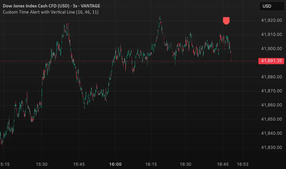
Custom Time Alert with Vertical Line📌 Detailed Explanation of the Custom Time Alert with Vertical Line in Pine Script v5
This script is a time-based alert system designed for TradingView. It allows traders to set a specific hour and minute for alerts and provides visual indicators on the chart, including a marker when the alert triggers and a vertical line at the alert time.
🔹 Main Features
Custom Alert Time → Users can specify the exact hour and minute for an alert.
Time Zone Offset Support → Users can manually adjust their local UTC offset to ensure alerts trigger at the correct time.
Real-Time Alert Condition → When the market reaches the set time, an alert notification is triggered.
Chart Visualization → A red marker appears when the alert is activated, and a blue vertical line is drawn at the alert time.
Automated Calculation → The script adjusts the alert time based on the user’s time zone settings.
🛠️ How It Works
User Input for Alert Time
The script allows users to enter their desired alert hour (0-23) and minute (0-59).
This ensures the alert triggers at the exact specified time.
Time Zone Offset Handling
Users enter their UTC offset (e.g., New York is -5, Tokyo is +9).
This ensures alerts work correctly regardless of the user’s location.
Time Calculation
The script adjusts the TradingView time by adding the time zone offset in milliseconds.
This converts the UTC-based TradingView time into the user’s local time.
Checking for a Time Match
The script constantly checks if the current hour and minute match the user-defined alert time.
If they match, the script activates an alert.
Triggering Alerts
The script uses TradingView’s alertcondition() function to create an alert.
When the time matches, TradingView sends a notification (e.g., pop-up, sound, or mobile alert).
Chart Markers for Visual Alerts
A red marker is displayed on the chart when the alert triggers.
A blue vertical line is drawn at the exact alert time.
📌 Example Use Cases
📈 1. Forex Traders Monitoring Market Opens
A forex trader who trades the London session wants an alert when the market opens at 8:00 AM UTC.
The trader sets:
Alert Hour = 8
Alert Minute = 0
Time Zone Offset = 0 (for UTC)
When the market reaches 8:00 AM UTC, the script triggers an alert.
📈 2. Stock Market Open Alerts
A trader in New York (EST) wants an alert at 9:30 AM Eastern Time (New York Stock Exchange open).
New York’s UTC offset is -5.
The trader sets:
Alert Hour = 9
Alert Minute = 30
Time Zone Offset = -5
The script ensures the alert triggers at 9:30 AM EST.
📈 3. Crypto Trader Watching a Specific Time
A crypto trader wants an alert for a specific strategy at 3:00 PM in Tokyo (UTC+9).
Tokyo’s UTC offset is +9.
The trader sets:
Alert Hour = 15
Alert Minute = 0
Time Zone Offset = +9
The script ensures the alert triggers exactly at 3:00 PM Tokyo time.
Divergence IQ [TradingIQ]Hello Traders!
Introducing "Divergence IQ"
Divergence IQ lets traders identify divergences between price action and almost ANY TradingView technical indicator. This tool is designed to help you spot potential trend reversals and continuation patterns with a range of configurable features.
Features
Divergence Detection
Detects both regular and hidden divergences for bullish and bearish setups by comparing price movements with changes in the indicator.
Offers two detection methods: one based on classic pivot point analysis and another that provides immediate divergence signals.
Option to use closing prices for divergence detection, allowing you to choose the data that best fits your strategy.
Normalization Options:
Includes multiple normalization techniques such as robust scaling, rolling Z-score, rolling min-max, or no normalization at all.
Adjustable normalization window lets you customize the indicator to suit various market conditions.
Option to display the normalized indicator on the chart for clearer visual comparison.
Allows traders to take indicators that aren't oscillators, and convert them into an oscillator - allowing for better divergence detection.
Simulated Trade Management:
Integrates simulated trade entries and exits based on divergence signals to demonstrate potential trading outcomes.
Customizable exit strategies with options for ATR-based or percentage-based stop loss and profit target settings.
Automatically calculates key trade metrics such as profit percentage, win rate, profit factor, and total trade count.
Visual Enhancements and On-Chart Displays:
Color-coded signals differentiate between bullish, bearish, hidden bullish, and hidden bearish divergence setups.
On-chart labels, lines, and gradient flow visualizations clearly mark divergence signals, entry points, and exit levels.
Configurable settings let you choose whether to display divergence signals on the price chart or in a separate pane.
Performance Metrics Table:
A performance table dynamically displays important statistics like profit, win rate, profit factor, and number of trades.
This feature offers an at-a-glance assessment of how the divergence-based strategy is performing.
The image above shows Divergence IQ successfully identifying and trading a bullish divergence between an indicator and price action!
The image above shows Divergence IQ successfully identifying and trading a bearish divergence between an indicator and price action!
The image above shows Divergence IQ successfully identifying and trading a hidden bullish divergence between an indicator and price action!
The image above shows Divergence IQ successfully identifying and trading a hidden bearish divergence between an indicator and price action!
The performance table is designed to provide a clear summary of simulated trade results based on divergence setups. You can easily review key metrics to assess the strategy’s effectiveness over different time periods.
Customization and Adaptability
Divergence IQ offers a wide range of configurable settings to tailor the indicator to your personal trading approach. You can adjust the lookback and lookahead periods for pivot detection, select your preferred method for normalization, and modify trade exit parameters to manage risk according to your strategy. The tool’s clear visual elements and comprehensive performance metrics make it a useful addition to your technical analysis toolbox.
The image above shows Divergence IQ identifying divergences between price action and OBV with no normalization technique applied.
While traders can look for divergences between OBV and price, OBV doesn't naturally behave like an oscillator, with no definable upper and lower threshold, OBV can infinitely increase or decrease.
With Divergence IQ's ability to normalize any indicator, traders can normalize non-oscillator technical indicators such as OBV, CVD, MACD, or even a moving average.
In the image above, the "Robust Scaling" normalization technique is selected. Consequently, the output of OBV has changed and is now behaving similar to an oscillator-like technical indicator. This makes spotting divergences between the indicator and price easier and more appropriate.
The three normalization techniques included will change the indicator's final output to be more compatible with divergence detection.
This feature can be used with almost any technical indicator.
Stop Type
Traders can select between ATR based profit targets and stop losses, or percentage based profit targets and stop losses.
The image above shows options for the feature.
Divergence Detection Method
A natural pitfall of divergence trading is that it generally takes several bars to "confirm" a divergence. This makes trading the divergence complicated, because the entry at time of the divergence might look great; however, the divergence wasn't actually signaled until several bars later.
To circumvent this issue, Divergence IQ offers two divergence detection mechanisms.
Pivot Detection
Pivot detection mode is the same as almost every divergence indicator on TradingView. The Pivots High Low indicator is used to detect market/indicator highs and lows and, consequently, divergences.
This method generally finds the "best looking" divergences, but will always take additional time to confirm the divergence.
Immediate Detection
Immediate detection mode attempts to reduce lag between the divergence and its confirmation to as little as possible while avoiding repainting.
Immediate detection mode still uses the Pivots Detection model to find the first high/low of a divergence. However, the most recent high/low does not utilize the Pivot Detection model, and instead immediately looks for a divergence between price and an indicator.
Immediate Detection Mode will always signal a divergence one bar after it's occurred, and traders can set alerts in this mode to be alerted as soon as the divergence occurs.
TradingView Backtester Integration
Divergence IQ is fully compatible with the TradingView backtester!
Divergence IQ isn’t designed to be a “profitable strategy” for users to trade. Instead, the intention of including the backtester is to let users backtest divergence-based trading strategies between the asset on their chart and almost any technical indicator, and to see if divergences have any predictive utility in that market.
So while the backtester is available in Divergence IQ, it’s for users to personally figure out if they should consider a divergence an actionable insight, and not a solicitation that Divergence IQ is a profitable trading strategy. Divergence IQ should be thought of as a Divergence backtesting toolkit, not a full-feature trading strategy.
Strategy Properties Used For Backtest
Initial Capital: $1000 - a realistic amount of starting capital that will resonate with many traders
Amount Per Trade: 5% of equity - a realistic amount of capital to invest relative to portfolio size
Commission: 0.02% - a conservative amount of commission to pay for trade that is standard in crypto trading, and very high for other markets.
Slippage: 1 tick - appropriate for liquid markets, but must be increased in markets with low activity.
Once more, the backtester is meant for traders to personally figure out if divergences are actionable trading signals on the market they wish to trade with the indicator they wish to use.
And that's all!
If you have any cool features you think can benefit Divergence IQ - please feel free to share them!
Thank you so much TradingView community!

is_strategyCorrection-Adaptive Trend Strategy (Open-Source)
Core Advantage: Designed specifically for the is_correction indicator, with full transparency and customization options.
Key Features:
Open-Source Code:
✅ Full access to the strategy logic – study how every trade signal is generated.
✅ Freedom to customize – modify entry/exit rules, risk parameters, or add new indicators.
✅ No black boxes – understand and trust every decision the strategy makes.
Built for is_correction:
Filters out false signals during market noise.
Works only in confirmed trends (is_correction = false).
Adaptable for Your Needs:
Change Take Profit/Stop Loss ratios directly in the code.
Add alerts, notifications, or integrate with other tools (e.g., Volume Profile).
For Developers/Traders:
Use the code as a template for your own strategies.
Test modifications risk-free on historical data.
How the Strategy Works:
Main Goal:
Automatically buys when the price starts rising and sells when it starts falling, but only during confirmed trends (ignoring temporary pullbacks).
What You See on the Chart:
📈 Up arrows ▼ (below the candle) = Buy signal.
📉 Down arrows ▲ (above the candle) = Sell signal.
Gray background = Market is in a correction (no trades).
Key Mechanics:
Buy Condition:
Price closes higher than the previous candle + is_correction confirms the main trend (not a pullback).
Example: Red candle → green candle → ▼ arrow → buy.
Sell Condition:
Price closes lower than the previous candle + is_correction confirms the trend (optional: turn off short-selling in settings).
Exit Rules:
Closes trades automatically at:
+0.5% profit (adjustable in settings).
-0.5% loss (adjustable).
Or if a reverse signal appears (e.g., sell signal after a buy).
User-Friendly Settings:
Sell – On (default: ON):
ON → Allows short-selling (selling when price falls).
OFF → Strategy only buys and closes positions.
Revers (default: OFF):
ON → Inverts signals (▼ = sell, ▲ = buy).
%Profit & %Loss:
Adjust these values (0-30%) to increase/decrease profit targets and risk.
Example Scenario:
Buy Signal:
Price rises for 3 days → green ▼ arrow → strategy buys.
Stop loss set 0.5% below entry price.
If price keeps rising → trade closes at +0.5% profit.
Correction Phase:
After a rally, price drops for 1 day → gray background → strategy ignores the drop (no action).
Stop Loss Trigger:
If price drops 0.5% from entry → trade closes automatically.
Key Features:
Correction Filter (is_correction):
Acts as a “noise filter” → avoids trades during temporary pullbacks.
Flexibility:
Disable short-selling, flip signals, or tweak profit/loss levels in seconds.
Transparency:
Open-source code → see exactly how every signal is generated (click “Source” in TradingView).
Tips for Beginners:
Test First:
Run the strategy on historical data (click the “Chart” icon in TradingView).
See how it performed in the past.
Customize It:
Increase %Profit to 2-3% for volatile assets like crypto.
Turn off Sell – On if short-selling confuses you.
Trust the Stop Loss:
Even if you think the price will rebound, the strategy will close at -0.5% to protect your capital.
Where to Find Settings:
Click the strategy name on the top-left of your chart → adjust sliders/toggles in the menu.
Русская Версия
Трендовая стратегия с открытым кодом
Главное преимущество: Полная прозрачность логики и адаптация под ваши нужды.
Особенности:
Открытый исходный код:
✅ Видите всю «кухню» стратегии – как формируются сигналы, когда открываются сделки.
✅ Меняйте правила – корректируйте тейк-профит, стоп-лосс или добавляйте новые условия.
✅ Никаких секретов – вы контролируете каждое правило.
Заточка под is_correction:
Игнорирует ложные сигналы в коррекциях.
Работает только в сильных трендах (is_correction = false).
Гибкая настройка:
Подстройте параметры под свой риск-менеджмент.
Добавьте свои индикаторы или условия для входа.
Для трейдеров и разработчиков:
Используйте код как основу для своих стратегий.
Тестируйте изменения на истории перед реальной торговлей.
Простыми словами:
Почему это удобно:
Открытый код = полный контроль. Вы можете:
Увидеть, как именно стратегия решает купить или продать.
Изменить правила закрытия сделок (например, поставить TP=2% вместо 1.5%).
Добавить новые условия (например, торговать только при высоком объёме).
Примеры кастомизации:
Новички: Меняйте только TP/SL в настройках (без кодинга).
Продвинутые: Добавьте RSI-фильтр, чтобы избегать перекупленности.
Разработчики: Встройте стратегию в свою торговую систему.
Как начать:
Скачайте код из TradingView.
Изучите логику в разделе strategy.entry/exit.
Меняйте параметры в блоке input.* (безопасно!).
Тестируйте изменения и оптимизируйте под свои цели.
Как работает стратегия:
Главная задача:
Автоматически покупает, когда цена начинает расти, и продаёт, когда падает. Но делает это «умно» — только когда рынок в основном тренде, а не во временном откате (коррекции).
Что видно на графике:
📈 Стрелки вверх ▼ (под свечой) — сигнал на покупку.
📉 Стрелки вниз ▲ (над свечой) — сигнал на продажу.
Серый фон — рынок в коррекции (не торгуем).
Как это работает:
Когда покупаем:
Если цена закрылась выше предыдущей и индикатор is_correction показывает «основной тренд» (не коррекция).
Пример: Была красная свеча → стала зелёная → появилась стрелка ▼ → покупаем.
Когда продаём:
Если цена закрылась ниже предыдущей и is_correction подтверждает тренд (опционально, можно отключить в настройках).
Когда закрываем сделку:
Автоматически при достижении:
+0.5% прибыли (можно изменить в настройках).
-0.5% убытка (можно изменить).
Или если появился противоположный сигнал (например, после покупки пришла стрелка продажи).
Настройки для чайников:
«Sell – On» (включено по умолчанию):
Если включено → стратегия будет продавать в шорт.
Если выключено → только покупки и закрытие позиций.
«Revers» (выключено по умолчанию):
Если включить → стратегия будет работать наоборот (стрелки ▼ = продажа, ▲ = покупка).
«%Profit» и «%Loss»:
Меняйте эти цифры (от 0 до 30), чтобы увеличить/уменьшить прибыль и риски.
Пример работы:
Сигнал на покупку:
Цена 3 дня растет → появляется зелёная стрелка ▼ → стратегия покупает.
Стоп-лосс ставится на 0.5% ниже цены входа.
Если цена продолжает расти → сделка закрывается при +0.5% прибыли.
Коррекция:
После роста цена падает на 1 день → фон становится серым → стратегия игнорирует это падение (не закрывает сделку).
Стоп-лосс:
Если цена упала на 0.5% от точки входа → сделка закрывается автоматически.
Важные особенности:
Фильтр коррекций (is_correction):
Это «защита от шума» — стратегия не реагирует на мелкие откаты, работая только в сильных трендах.
Гибкие настройки:
Можно запретить шорты, перевернуть сигналы или изменить уровни прибыли/убытка за 2 клика.
Прозрачность:
Весь код открыт → вы можете увидеть, как формируется каждый сигнал (меню «Исходник» в TradingView).
Советы для новичков:
Начните с теста:
Запустите стратегию на исторических данных (кнопка «Свеча» в окне TradingView).
Посмотрите, как она работала в прошлом.
Настройте под себя:
Увеличьте %Profit до 2-3%, если торгуете валюты.
Отключите «Sell – On», если не понимаете шорты.
Доверяйте стоп-лоссу:
Даже если кажется, что цена развернётся — стратегия закроет сделку при -0.5%, защитив ваш депозит.
Где найти настройки:
Кликните на название стратегии в верхнем левом углу графика → откроется меню с ползунками и переключателями.
Важно: Стратегия предоставляет «рыбу» – чтобы она стала «уловистой», адаптируйте её под свой стиль торговли!

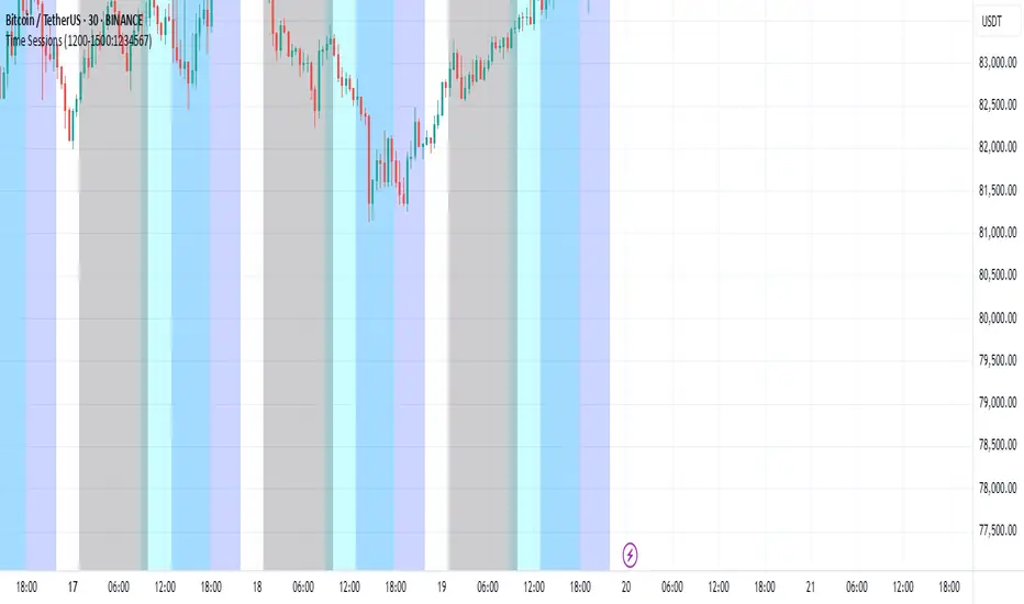
Timeframe Display + Countdown📘 Help Guide: Timeframe Display + Countdown + Alert
🔹 Overview
This indicator displays:
✅ The selected timeframe (e.g., 5min, 1H, 4H)
✅ A countdown timer showing minutes and seconds until the current candle closes
✅ An optional alert that plays a sound when 1 minute remains before the new candle starts
⚙️ How to Use
1️⃣ Add the Indicator
• Open TradingView
• Click on Pine Script Editor
• Copy and paste the script
• Click Add to Chart
2️⃣ Customize Settings
• Text Color: Choose a color for the displayed text
• Text Size: Adjust the font size (8–24)
• Transparency: Set how transparent the text is (0%–100%)
• Position: Choose where the text appears (Top Left, Top Right, Bottom Left, Bottom Right)
• Enable Audible Alert: Turn ON/OFF the alert when 1 minute remains
3️⃣ Set Up an Audible Alert in TradingView
🚨 Important: Pine Script cannot play sounds directly; you must set up a manual alert in TradingView.
Steps:
1. Click “Alerts” (🔔 icon in TradingView)
2. Click “Create Alert” (+ button)
3. In “Condition”, select this indicator (Timeframe Display + Countdown)
4. Under “Options”, choose:
• Trigger: “Once Per Bar”
• Expiration: Set a valid time range
• Alert Actions: Check “Play Sound” and choose a sound
5. Click “Create” ✅
🛠️ How It Works
• Countdown Timer:
• Updates in real time, displaying MM:SS until the candle closes
• Resets when a new candle starts
• Alert Trigger:
• When 1:00 minute remains, an alert is sent
• If properly configured in TradingView, it plays a sound

Volume Delta with Bollinger Bands [EMA]TL;DR
This indicator displays a “Volume Delta” candle chart based on a lower timeframe approximation of up vs. down volume. Bollinger Bands (using an EMA and a configurable standard deviation multiplier) highlight when Volume Delta exceeds typical volatility thresholds. Green bars will darken when Volume Delta is above the upper Bollinger band, and red bars will darken when Volume Delta is below the lower Bollinger band. You can optionally include wicks in the Bollinger calculations. Note : TradingView uses tick-based volume data, so these values may not precisely match true market orders.
What Is Volume Delta ?
• Volume Delta is a metric that identifies buying vs. selling activity in a market by distinguishing between orders transacting at the ask (buy volume) and orders transacting at the bid (sell volume).
• A positive Volume Delta indicates more buy volume during a bar, while a negative Volume Delta indicates more sell volume.
How TradingView Calculates Volume Delta
• TradingView relies on tick data to approximate up/down volume. This may not perfectly capture true order-flow distribution, particularly on higher timeframes or illiquid symbols.
• While it can provide useful insights into volume flow, keep in mind the underlying data’s limitations.
Key Features of This Indicator
1. Automatic or Custom Lower Timeframe Data
• The script can automatically select a lower timeframe for Volume Delta, or you can manually specify one in the settings.
2. Bollinger Bands on Volume Delta
• Uses an EMA of the Volume Delta (or a wick-based average) and calculates a standard deviation.
• The upper and lower bands highlight when activity deviates from typical volatility.
3. Configurable Wick Inclusion
• Decide whether to use only the “close” (lastVolume) of the Volume Delta bar or the average of its wicks ((maxVolume + minVolume) / 2) for Bollinger calculations.
4. Dynamic Bar Colors
• Positive Volume Delta bars turn dark green if they exceed the upper Bollinger band, otherwise lighter green .
• Negative Volume Delta bars turn dark red if they fall below the lower Bollinger band, otherwise lighter red .
How To Use
1. Add the Indicator to Your Chart
• Apply it to any symbol and timeframe in TradingView.
• Configure the lower timeframe for Volume Delta if desired.
2. Adjust Bollinger Settings
• Bollinger Length defines the EMA and standard deviation period.
• Bollinger Multiplier sets how far the bands lie from the EMA.
3. Choose Whether To Use Wicks
• Toggle to use the average of high/low for a potentially more volatile reading.
• Turn it off to rely solely on the Volume Delta “close.”
4. Interpret the Signals
• Dark Green Above the Upper Band : Suggests strong buying pressure above normal.
• Lighter Green : Positive but within typical volatility bounds.
• Dark Red Below the Lower Band : Suggests strong selling pressure below normal.
• Lighter Red : Negative but within typical volatility.
Important Caveats
• TradingView Volume Data : Tick-based and aggregated data may not reflect actual order-flow precisely.
• Context Matters : Combine Volume Delta with other forms of analysis (price action, support/resistance, etc.) to form a more comprehensive strategy.
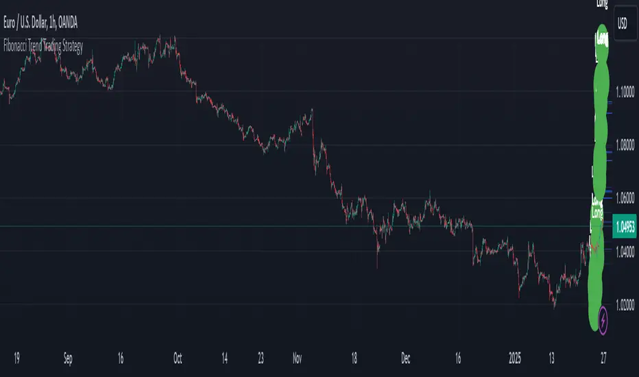
Fibonacci Extension Strt StrategyCore Logic and Steps:
Weekly Trend Identification:
Find the last significant Higher High (HH) and Lower Low (LL) or vice-versa on the Weekly timeframe.
Determine if it's an uptrend (HH followed by LL) or a downtrend (LL followed by HH).
Plot a Fibonacci Extension (or Retracement in reverse order) from the swing point determined to the other significant swing point.
Weekly Retracement Levels:
Display horizontal lines at the 0.236, 0.382, and 0.5 Fibonacci levels from the weekly extension.
Monitor price action on these levels.
Daily Confirmation:
When price hits the Fib levels, examine the Daily chart.
Look for a rejection wick (indicating the pull back is ending) on the identified weekly retracement levels.
Confirm that the price is indeed starting to continue in the direction of the original weekly trend.
Four-Hour Entry:
On the 4H timeframe, plot a new Fib Extension in the opposite direction of the weekly.
If it's an uptrend, the Fib is plotted from last swing low to its swing high. If the weekly trend was bearish the Fib will be plotted from last swing high to the swing low.
Generate an entry when price breaks the high of that candle.
Trade Management:
Entry is on the breakout of the current candle.
Stop Loss: Place the stop loss below the wick of the breakout candle.
Take Profit 1: Close 50% of the position at the 0.5 Fibonacci level. Move the stop loss to breakeven on this position.
Take Profit 2: Close another 25% of the position at the 0.236 Fib level.
Trailing Take Profit: Keep the last 25% open, using a trailing stop loss. (You'll need to define the logic for the trailing stop, e.g., trailing stop using the last high/low)
How to Use in TradingView:
Open a TradingView Chart.
Click on "Pine Editor" at the bottom.
Copy and paste the corrected Pine Script code.
Click "Add to Chart".
The indicator should now be displayed on your chart.
Bollinger Bands CustomThe indicator is a customized version of Bollinger Bands with added trading signals. This indicator is designed to help traders identify potential entry (buy) and exit (sell) points based on the interaction between the price and the Bollinger Bands. Below, I will explain in detail its purpose, how it works, and how to use it.
Purpose of the Indicator
The main purpose of this indicator is:
Identify market volatility: Bollinger Bands expand and contract based on price volatility.
Provide trading signals: The indicator generates buy signals (BUY) when the price crosses the lower band and sell signals (SELL) when the price crosses the upper band.
Help identify dynamic support and resistance levels: The upper and lower bands act as dynamic resistance and support levels.
How the Indicator Works
The indicator is based on three main components:
Moving Average (SMA): It calculates the simple moving average (SMA) of the price over a specified period (length).
Bollinger Bands:
The upper band is calculated as the moving average plus a standard deviation multiplied by a factor (mult).
The lower band is calculated as the moving average minus a standard deviation multiplied by the same factor.
Trading signals:
A BUY signal is generated when the price crosses above the lower band.
A SELL signal is generated when the price crosses below the upper band.
How to Use the Indicator
Here is a step-by-step guide on how to use the indicator on TradingView:
1. Add the Indicator to the Chart
Copy the Pine Script code you created.
Open TradingView and go to the Pine Editor.
Paste the code and click "Add to Chart."
The indicator will be displayed directly on the price chart.
2. Customize the Parameters
You can customize the following parameters:
Moving Average Length (length): Set the period for the moving average (default is 20).
Price Source (source): Choose the price to use (default is the closing price).
Standard Deviation Multiplier (mult): Set the multiplier for the standard deviation (default is 2.0).
3. Interpret the Signals
BUY Signal: When you see a "BUY" label below a candle, it means the price has crossed above the lower band. This could indicate a buying opportunity.
SELL Signal: When you see a "SELL" label above a candle, it means the price has crossed below the upper band. This could indicate a selling opportunity.
4. Use Bollinger Bands as Support and Resistance
If the price approaches the upper band, it might indicate a resistance level.
If the price approaches the lower band, it might indicate a support level.
5. Monitor the Colored Background
The chart background turns light green when there is a BUY signal and light red when there is a SELL signal. This helps you quickly identify signals.
Practical Example
Suppose you are analyzing a daily chart of a stock or cryptocurrency:
If the price crosses above the lower band, the indicator will show a "BUY" label. You might consider this as a signal to open a long position.
If the price crosses below the upper band, the indicator will show a "SELL" label. You might consider this as a signal to close a long position or open a short position.
Limitations and Considerations
False signals: In range-bound markets, Bollinger Bands can generate many false signals. It is advisable to use this indicator in combination with other technical analysis tools.
Extreme volatility: During periods of high volatility, the bands expand, and signals may become less reliable.
Confirmation: It is always good practice to confirm signals with other indicators (e.g., RSI, MACD) or candlestick analysis.
Conclusion
My indicator is a useful tool for identifying potential trading opportunities based on Bollinger Bands. However, as with any indicator, it is important to use it in combination with other forms of analysis and risk management to maximize effectiveness. Happy trading! 🚀

RSI from Rolling VWAP [CHE]Introducing the RSI from Rolling VWAP Indicator
Elevate your trading strategy with the RSI from Rolling VWAP —a cutting-edge indicator designed to provide unparalleled insights and enhance your decision-making on TradingView. This advanced tool seamlessly integrates the Relative Strength Index (RSI) with a Rolling Volume-Weighted Average Price (VWAP) to deliver precise and actionable trading signals.
Why Choose RSI from Rolling VWAP ?
- Clear Trend Detection: Our enhanced algorithms ensure accurate identification of bullish and bearish trends, allowing you to capitalize on market movements with confidence.
- Customizable Time Settings: Tailor the time window in days, hours, and minutes to align perfectly with your unique trading strategy and market conditions.
- Flexible Moving Averages: Select from a variety of moving average types—including SMA, EMA, WMA, and more—to smooth the RSI, providing clearer trend analysis and reducing market noise.
- Threshold Alerts: Define upper and lower RSI thresholds to effortlessly spot overbought or oversold conditions, enabling timely and informed trading decisions.
- Visual Enhancements: Enjoy a visually intuitive interface with color-coded RSI lines, moving averages, and background fills that make interpreting market data straightforward and efficient.
- Automatic Signal Labels: Receive immediate bullish and bearish labels directly on your chart, signaling potential trading opportunities without the need for constant monitoring.
Key Features
- Inspired by Proven Tools: Building upon the robust foundation of TradingView's Rolling VWAP, our indicator offers enhanced functionality and greater precision.
- Volume-Weighted Insights: By incorporating volume into the VWAP calculation, gain a deeper understanding of price movements and market strength.
- User-Friendly Configuration: Easily adjust settings to match your trading preferences, whether you're a novice trader or an experienced professional.
- Hypothesis-Driven Analysis: Utilize hypothetical results to backtest strategies, understanding that past performance does not guarantee future outcomes.
How It Works
1. Data Integration: Utilizes the `hlc3` (average of high, low, and close) as the default data source, with customization options available to suit your trading needs.
2. Dynamic Time Window: Automatically calculates the optimal time window based on an auto timeframe or allows for fixed time periods, ensuring flexibility and adaptability.
3. Rolling VWAP Calculation: Accurately computes the Rolling VWAP by balancing price and volume over the specified time window, providing a reliable benchmark for price action.
4. RSI Analysis: Measures momentum through RSI based on Rolling VWAP changes, smoothed with your chosen moving average for enhanced trend clarity.
5. Actionable Signals: Detects and labels bullish and bearish conditions when RSI crosses predefined thresholds, offering clear indicators for potential market entries and exits.
Seamless Integration with Your TradingView Experience
Adding the RSI from Rolling VWAP to your TradingView charts is straightforward:
1. Add to Chart: Simply copy the Pine Script code into TradingView's Pine Editor and apply it to your desired chart.
2. Customize Settings: Adjust the Source Settings, Time Settings, RSI Settings, MA Settings, and Color Settings to align with your trading strategy.
3. Monitor Signals: Watch for RSI crossings above or below your set thresholds, accompanied by clear labels indicating bullish or bearish trends.
4. Optimize Your Trades: Leverage the visual and analytical strengths of the indicator to make informed buy or sell decisions, maximizing your trading potential.
Disclaimer:
The content provided, including all code and materials, is strictly for educational and informational purposes only. It is not intended as, and should not be interpreted as, financial advice, a recommendation to buy or sell any financial instrument, or an offer of any financial product or service. All strategies, tools, and examples discussed are provided for illustrative purposes to demonstrate coding techniques and the functionality of Pine Script within a trading context.
Any results from strategies or tools provided are hypothetical, and past performance is not indicative of future results. Trading and investing involve high risk, including the potential loss of principal, and may not be suitable for all individuals. Before making any trading decisions, please consult with a qualified financial professional to understand the risks involved.
By using this script, you acknowledge and agree that any trading decisions are made solely at your discretion and risk.
Get Started Today
Transform your trading approach with the RSI from Rolling VWAP indicator. Experience the synergy of momentum and volume-based analysis, and unlock the potential for more accurate and profitable trades.
Download now and take the first step towards a more informed and strategic trading journey!
For further inquiries or support, feel free to contact
Best regards
Chervolino
Inspired by the acclaimed Rolling VWAP by TradingView
$TUBR: Stop Loss IndicatorATR-Based Stop Loss Indicator for TradingView by The Ultimate Bull Run Community: TUBR
**Overview**
The ATR-Based Stop Loss Indicator is a custom tool designed for traders using TradingView. It helps you determine optimal stop loss levels by leveraging the Average True Range (ATR), a popular measure of market volatility. By adapting to current market conditions, this indicator aims to minimize premature stop-outs and enhance your risk management strategy.
---
**Key Features**
- **Dynamic Stop Loss Levels**: Calculates stop loss prices based on the ATR, providing both long and short stop loss suggestions.
- **Customizable Parameters**: Adjust the ATR period, multiplier, and smoothing method to suit your trading style and the specific instrument you're trading.
- **Visual Aids**: Plots stop loss lines directly on your chart for easy visualization.
- **Alerts and Notifications** (Optional): Set up alerts to notify you when the price approaches or hits your stop loss levels.
---
**Understanding the Indicator**
1. **Average True Range (ATR)**:
- **What It Is**: ATR measures market volatility by calculating the average range between high and low prices over a specified period.
- **Why It's Useful**: A higher ATR indicates higher volatility, which can help you set stop losses that accommodate market fluctuations.
2. **ATR Multiplier**:
- **Purpose**: Determines how far your stop loss is placed from the current price based on the ATR.
- **Example**: An ATR multiplier of 1.5 means the stop loss is set at 1.5 times the ATR away from the current price.
3. **Smoothing Methods**:
- **Options**: Choose from RMA (default), SMA, EMA, WMA, or Hull MA.
- **Effect**: Different smoothing methods can make the ATR more responsive or smoother, affecting where the stop loss is placed.
---
**How the Indicator Works**
- **Long Stop Loss Calculation**:
- **Formula**: `Long Stop Loss = Close Price - (ATR * ATR Multiplier)`
- **Purpose**: For long positions, the stop loss is set below the current price to protect against downside risk.
- **Short Stop Loss Calculation**:
- **Formula**: `Short Stop Loss = Close Price + (ATR * ATR Multiplier)`
- **Purpose**: For short positions, the stop loss is set above the current price to protect against upside risk.
- **Plotting on the Chart**:
- **Green Line**: Represents the suggested stop loss level for long positions.
- **Red Line**: Represents the suggested stop loss level for short positions.
---
**How to Use the Indicator**
1. **Adding the Indicator to Your Chart**:
- **Step 1**: Copy the PineScript code of the indicator.
- **Step 2**: In TradingView, click on **Pine Editor** at the bottom of the platform.
- **Step 3**: Paste the code into the editor and click **Add to Chart**.
- **Step 4**: The indicator will appear on your chart with the default settings.
2. **Adjusting the Settings**:
- **ATR Period**:
- **Definition**: Number of periods over which the ATR is calculated.
- **Adjustment**: Increase for a smoother ATR; decrease for a more responsive ATR.
- **ATR Multiplier**:
- **Definition**: Factor by which the ATR is multiplied to set the stop loss distance.
- **Adjustment**: Increase to widen the stop loss (less likely to be hit); decrease to tighten the stop loss.
- **Smoothing Method**:
- **Options**: RMA, SMA, EMA, WMA, Hull MA.
- **Adjustment**: Experiment to see which method aligns best with your trading strategy.
- **Display Options**:
- **Show Long Stop Loss**: Toggle to display or hide the long stop loss line.
- **Show Short Stop Loss**: Toggle to display or hide the short stop loss line.
3. **Interpreting the Indicator**:
- **Long Positions**:
- **Action**: Set your stop loss at the value indicated by the green line when entering a long trade.
- **Short Positions**:
- **Action**: Set your stop loss at the value indicated by the red line when entering a short trade.
- **Adjusting Stop Losses**:
- **Trailing Stops**: You may choose to adjust your stop loss over time, moving it in the direction of your trade as the ATR-based stop loss levels change.
4. **Implementing in Your Trading Strategy**:
- **Risk Management**:
- **Position Sizing**: Use the stop loss distance to calculate your position size based on your risk tolerance.
- **Consistency**: Apply the same settings consistently to maintain discipline.
- **Combining with Other Indicators**:
- **Enhance Decision-Making**: Use in conjunction with trend indicators, support and resistance levels, or other technical analysis tools.
- **Alerts Setup** (If included in the code):
- **Purpose**: Receive notifications when the price approaches or hits your stop loss level.
- **Configuration**: Set up alerts in TradingView based on the alert conditions defined in the indicator.
---
**Benefits of Using This Indicator**
- **Adaptive Risk Management**: By accounting for current market volatility, the indicator helps prevent setting stop losses that are too tight or too wide.
- **Minimize Premature Stop-Outs**: Reduces the likelihood of being stopped out due to normal price fluctuations.
- **Flexibility**: Customizable settings allow you to tailor the indicator to different trading instruments and timeframes.
- **Visualization**: Clear visual representation of stop loss levels aids in quick decision-making.
---
**Things to Consider**
- **Market Conditions**:
- **High Volatility**: Be cautious as ATR values—and thus stop loss distances—can widen, increasing potential losses.
- **Low Volatility**: Tighter stop losses may increase the chance of being stopped out by minor price movements.
- **Backtesting and Optimization**:
- **Historical Analysis**: Test the indicator on past data to evaluate its effectiveness and adjust settings accordingly.
- **Continuous Improvement**: Regularly reassess and fine-tune the parameters to adapt to changing market conditions.
- **Risk Per Trade**:
- **Alignment with Risk Tolerance**: Ensure the stop loss level keeps potential losses within your acceptable risk per trade (e.g., 1-2% of your trading capital).
- **Emotional Discipline**:
- **Stick to Your Plan**: Avoid making impulsive changes to your stop loss levels based on emotions rather than analysis.
---
**Example Usage Scenario**
1. **Setting Up a Long Trade**:
- **Entry Price**: $100
- **ATR Value**: $2
- **ATR Multiplier**: 1.5
- **Calculated Stop Loss**: $100 - ($2 * 1.5) = $97
- **Action**: Place a stop loss order at $97.
2. **During the Trade**:
- **Price Increases to $105**
- **ATR Remains at $2**
- **New Stop Loss Level**: $105 - ($2 * 1.5) = $102
- **Action**: Move your stop loss up to $102 to lock in profits.
---
**Final Tips**
- **Documentation**: Keep a trading journal to record your trades, stop loss levels, and observations for future reference.
- **Education**: Continuously educate yourself on risk management and technical analysis to enhance your trading skills.
- **Support**: Engage with trading communities or seek professional advice if you're unsure about implementing the indicator effectively.
---
**Conclusion**
The ATR-Based Stop Loss Indicator is a valuable tool for traders looking to enhance their risk management by setting stop losses that adapt to market volatility. By integrating this indicator into your trading routine, you can improve your ability to protect capital and potentially increase profitability. Remember to use it as part of a comprehensive trading strategy, and always adhere to sound risk management principles.
---
**How to Access the Indicator**
To start using the ATR-Based Stop Loss Indicator, follow these steps:
1. **Obtain the Code**: Copy the PineScript code provided for the indicator.
2. **Create a New Indicator in TradingView**:
- Open TradingView and navigate to the **Pine Editor**.
- Paste the code into the editor.
- Click **Save** and give your indicator a name.
3. **Add to Chart**: Click **Add to Chart** to apply the indicator to your current chart.
4. **Customize Settings**: Adjust the input parameters to suit your preferences and start integrating the indicator into your trading strategy.
---
**Disclaimer**
Trading involves significant risk, and it's possible to lose all your capital. The ATR-Based Stop Loss Indicator is a tool to aid in decision-making but does not guarantee profits or prevent losses. Always conduct your own analysis and consider seeking advice from a financial professional before making trading decisions.

Volatility Adaptive Signal Tracker (VAST)The Adaptive Trend Following Buy/Sell Signals Pine Script is designed to help traders identify and capitalize on market trends using an adaptive trend-following strategy. This script focuses on generating reliable buy and sell signals by analyzing market trends and volatility. It simplifies the trading process by providing clear signals without plotting additional lines, making it easy to use and interpret.
Key Features:
Adaptive Trend Following:
The script employs an adaptive trend-following approach that leverages market volatility to generate buy and sell signals. This method is effective in both trending and volatile markets.
Inputs and Customization:
The script includes customizable parameters for the Simple Moving Average (SMA) length, the Average True Range (ATR) length, and the ATR multiplier. These inputs allow traders to adjust the sensitivity of the signals to match their trading style and market conditions.
Signal Generation:
Buy Signal: Generated when the closing price crosses above the upper adaptive band, indicating a potential upward trend.
Sell Signal: Generated when the closing price crosses below the lower adaptive band, indicating a potential downward trend.
Visual Signals:
The script uses plotshape to mark buy signals with green labels below the bars and sell signals with red labels above the bars. This clear visual representation helps traders quickly identify trading opportunities.
Alert Conditions:
The script sets up alert conditions for both buy and sell signals. Traders can use these alerts to receive notifications when a signal is generated, ensuring they do not miss any trading opportunities.
How It Works:
SMA Calculation: The script calculates the Simple Moving Average (SMA) over a specified period, which helps in identifying the general trend direction.
ATR Calculation: The Average True Range (ATR) is calculated to measure market volatility.
Adaptive Bands: Upper and lower adaptive bands are created by adding and subtracting a multiple of the ATR to the SMA, respectively.
Signal Logic: Buy signals are generated when the closing price crosses above the upper band, while sell signals are generated when the closing price crosses below the lower band.
Example Use Case:
A trader looking to capitalize on medium-term trends in the Nifty futures market can use this script to receive timely buy and sell signals. By customizing the SMA length and ATR parameters, the trader can fine-tune the script to match their trading strategy, ensuring they enter and exit trades at optimal points.
Benefits:
Simplicity: The script provides clear buy and sell signals without cluttering the chart with additional lines or indicators.
Adaptability: Customizable parameters allow traders to adapt the script to various market conditions and trading styles.
Alerts: Built-in alert conditions ensure traders receive timely notifications, helping them to act quickly on trading signals.
How to Use:
Open TradingView: Go to the TradingView website and log in.
Create a New Chart: Click on the “Chart” button to open a new chart.
Open the Pine Script Editor: Click on the “Pine Editor” tab at the bottom of the chart.
Create a New Script: Delete any default code in the Pine Script editor and paste the provided script.
Add to Chart: Click on the “Add to Chart” button to compile and add the script to your chart.
Save the Script: Click “Save” and name the script.
Set Alerts: Right-click on the chart, select “Add Alert,” and choose the appropriate condition to set alerts for buy and sell signals.

Gold Option Signals with EMA and RSIIndicators:
Exponential Moving Averages (EMAs): Faster to respond to recent price changes compared to simple moving averages.
RSI: Measures the magnitude of recent price changes to evaluate overbought or oversold conditions.
Signal Generation:
Buy Call Signal: Generated when the short EMA crosses above the long EMA and the RSI is not overbought (below 70).
Buy Put Signal: Generated when the short EMA crosses below the long EMA and the RSI is not oversold (above 30).
Plotting:
EMAs: Plotted on the chart to visualize trend directions.
Signals: Plotted as shapes on the chart where conditions are met.
RSI Background Color: Changes to red for overbought and green for oversold conditions.
Steps to Use:
Add the Script to TradingView:
Open TradingView, go to the Pine Script editor, paste the script, save it, and add it to your chart.
Interpret the Signals:
Buy Call Signal: Look for green labels below the price bars.
Buy Put Signal: Look for red labels above the price bars.
Customize Parameters:
Adjust the input parameters (e.g., lengths of EMAs, RSI levels) to better fit your trading strategy and market conditions.
Testing and Validation
To ensure that the script works as expected, you can test it on historical data and validate the signals against known price movements. Adjust the parameters if necessary to improve the accuracy of the signals.
azLibConnectorThe AzLibConnector provides a comprehensive suite of functions for facilitating seamless communication and chaining of signal value streams between connectable indicators, signal filters, monitors, and strategies on TradingView. By adeptly integrating both positive and negative weights from Entry Long (EL), Exit Long (XL), Entry Short (ES), and Exit Short (XS) signals into a singular figure, it leverages the source input field of TradingView to efficiently connect indicators in a chain. This results in a streamlined strategy setup without the necessity for Pine Script coding. Emphasizing modularity and uniformity, this library enables users to easily combine indicators into a coherent system, facilitating strategy development and execution with flexibility.
█ LIBRARY USAGE
extract(srcConnector)
Extract signals (EL, XL, ES, XS) from incoming connector signal stream
Parameters:
srcConnector : (series float) Source Connector. The connector stream series to extract the signals from.
Returns: A tuple containing the extracted EL, XL, ES, XS signal values.
compose(signalEL, signalXL, signalES, signalXS)
Compose a connector output signal stream from given EL, XL, ES and XS signals to be used by other Azullian Strategy Builder blocks.
Parameters:
signalEL : (series float) Entry Long signal value.
signalXL : (series float) Exit Long signal value.
signalES : (series float) Entry Short signal value.
signalXS : (series float) Exit Short signal value.
Returns: (series float) A composed connector output signal stream.
█ USAGE OF CONNECTABLE INDICATORS
■ Connectable chaining mechanism
Connectable indicators can be connected directly to the monitor, signal filter or strategy , or they can be daisy chained to each other while the last indicator in the chain connects to the monitor, signal filter or strategy. When using a signal filter or monitor you can chain the filter to the strategy input to make your chain complete.
• Direct chaining: Connect an indicator directly to the monitor, signal filter or strategy through the provided inputs (→).
• Daisy chaining: Connect indicators using the indicator input (→). The first in a daisy chain should have a flow (⌥) set to 'Indicator only'. Subsequent indicators use 'Both' to pass the previous weight. The final indicator connects to the monitor, signal filter, or strategy.
■ Set up the signal filter with a connectable indicator and strategy
Let's connect the MACD to a connectable signal filter and a strategy :
1. Load all relevant indicators
• Load MACD / Connectable
• Load Signal filter / Connectable
• Load Strategy / Connectable
2. Signal Filter: Connect the MACD to the Signal Filter
• Open the signal filter settings
• Choose one of the five input dropdowns (1→, 2→, 3→, 4→, 5→) and choose : MACD / Connectable: Signal Connector
• Toggle the enable box before the connected input to enable the incoming signal
3. Signal Filter: Update the filter settings if needed
• The default filter mode for the trading direction is SWING, and is compatible with the default settings in the strategy and indicators.
4. Signal Filter: Update the weight threshold settings if needed
• All connectable indicators load by default with a score of 6 for each direction (EL, XL, ES, XS)
• By default, weight threshold is 'ABOVE' Threshold 1 (TH1) and Threshold 2 (TH2), both set at 5. This allows each occurrence to score, as the default score is 1 point above the threshold.
5. Strategy: Connect the strategy to the signal filter in the strategy settings
• Select a strategy input → and select the Signal filter: Signal connector
6. Strategy: Enable filter compatible directions
• As the default setting of the filter is SWING, we should also set the SM (Strategy mode) to SWING.
Now that everything is connected, you'll notice green spikes in the signal filter or signal monitor representing long signals, and red spikes indicating short signals. Trades will also appear on the chart, complemented by a performance overview. Your journey is just beginning: delve into different scoring mechanisms, merge diverse connectable indicators, and craft unique chains. Instantly test your results and discover the potential of your configurations. Dive deep and enjoy the process!
█ BENEFITS
• Adaptable Modular Design: Arrange indicators in diverse structures via direct or daisy chaining, allowing tailored configurations to align with your analysis approach.
• Streamlined Backtesting: Simplify the iterative process of testing and adjusting combinations, facilitating a smoother exploration of potential setups.
• Intuitive Interface: Navigate TradingView with added ease. Integrate desired indicators, adjust settings, and establish alerts without delving into complex code.
• Signal Weight Precision: Leverage granular weight allocation among signals, offering a deeper layer of customization in strategy formulation.
• Advanced Signal Filtering: Define entry and exit conditions with more clarity, granting an added layer of strategy precision.
• Clear Visual Feedback: Distinct visual signals and cues enhance the readability of charts, promoting informed decision-making.
• Standardized Defaults: Indicators are equipped with universally recognized preset settings, ensuring consistency in initial setups across different types like momentum or volatility.
• Reliability: Our indicators are meticulously developed to prevent repainting. We strictly adhere to TradingView's coding conventions, ensuring our code is both performant and clean.
█ COMPATIBLE INDICATORS
Each indicator that incorporates our open-source 'azLibConnector' library and adheres to our conventions can be effortlessly integrated and used as detailed above.
For clarity and recognition within the TradingView platform, we append the suffix ' / Connectable' to every compatible indicator.
█ COMMON MISTAKES
• Removing an indicator from a chain: Deleting a linked indicator and confirming the "remove study tree" alert will also remove all underlying indicators in the object tree. Before removing one, disconnect the adjacent indicators and move it to the object stack's bottom.
• Point systems: The azLibConnector provides 500 points for each direction (EL: Enter long, XL: Exit long, ES: Enter short, XS: Exit short) Remember this cap when devising a point structure.
• Flow misconfiguration: In daisy chains the first indicator should always have a flow (⌥) setting of 'indicator only' while other indicator should have a flow (⌥) setting of 'both'.
█ A NOTE OF GRATITUDE
Through years of exploring TradingView and Pine Script, we've drawn immense inspiration from the community's knowledge and innovation. Thank you for being a constant source of motivation and insight.
█ RISK DISCLAIMER
Azullian's content, tools, scripts, articles, and educational offerings are presented purely for educational and informational uses. Please be aware that past performance should not be considered a predictor of future results.
5EMA BollingerBand Nifty Stock Scanner
What ?
We all heard about (well: over-heard) 5-EMA strategy. Which falls into the broader category of mean reversal type of trading setup.
What is mean reversal?
Price (or any time series, in fact) tries to follow a mean . Whenever price diverges from the mean it tries to meet it back.
It is empirically observed by some traders (I honestly don't know who first time observed it) that in Indian context specially, 5 Exponential Moving Average (5-EMA) works pretty good as that mean.
So whenever price moves away from that 5-EMA, it ultimately comes back and attain total nirvana :) Means: if price moved way higher than the 5EMA without touching it, then price will correct to meet it's 5-EMA and if price moved way lower, it will be uplifted to meet it's 5-EMA. Funny - but it works !
Now there are already enough social media coverage on this 5-EMA strategy/setup. Even TradingView has some excellent work done on these setups. Kudos to all those great souls.
So when we came to know about this, we were thinking what we should do for the community. Because it is well cover topic (specially in Indian context). Also, there are public indicators.
Then we thought why not come up with a scanner which will scan all the Nifty-50 constituent stocks and find out on the fly, real-time which all stocks are matching this 5-EMA setup and causing a Buy/Sell trade recommendation.
Hence here we are with the first version of our first scanner on the 5EMA setup (well it has some more masala than merely a 5-EMA setup).
Why?
Parts of why is already covered up.
Now instead of blindly following 5-EMA setup, we added the Bollinger band as well. Again: it's also not new. There are enough coverage in social media about the 5-EMA+BB strategy/setup. We mercilessly borrowed from all of these.
Suppose you have an indicator.
Now you apply the indicator in your chart. And then you need to (rock) and roll through your watchlist of Nifty-50 stocks (note: TradingView has no default watchlist of Nifty-50 stock by default - you have to create one custom watchlist to list all manually) to find out which all are matching the setup, need to take a note about the trade recomendations (entry, SL, target) and other stuffs like VWAP, Volume, volatility (Bollinger Band Width).
Not any more.
This scanner will track all the Nifty-50 stocks (technically: 40 stocks other than Banking stocks) and provide which one to Buy or Sell (if any), what's the entry, SL, target, where is the VWAP of the day, what's the picture in volume (high, low, rising, falling) and the implied volatility (using Bolling band width). Also it has a naive alerting mechanism as well.
In fact the code is there to monitor the (Future) OI also and all the OI drama (OI vs price and all the 4 stuffs like long build up, long unwinding, short covering, short buildup). But unfortunately, due to some limitations of the TradingView (that one can not monitor more than 40 `ta.security` call) we have to comment out the code. If you wish you can monitor only 20 stocks and enable the OI monitoring also (20 for stocks + 20 for their OI monitoring .. total 40 `ta.security` call).
How?
To know the divergence from 5-EMA we just check if the high of the candle (on closing) is below the 5-EMA. Then we check if the closing is inside the Bollinger Band (BB). That's a Buy signal. SL: low of the candle, T: middle and higher BB.
Just opposite for selling. 5-EMA low should be above 5-EMA and closing should be inside BB (lesser than BB higher level). That's a Sell signal. SL: high of the candle, T: middle and lower BB.
Along with we compare the current bar's volume with the last-20 bar VWMA (volume weighted moving average) to determine if the volume is high or low.
Present bar's volume is compared with the previous bar's volume to know if it's rising or falling.
VWAP is also determined using `ta.vwap` built-in support of TradingView.
The Bolling Band width is also notified, along with whether it is rising or falling (comparing with previous candle).
Simple, but effective.
Customization
As usual the EMA setup (5 default), the BB setup (20 SMA with 1.5 standard deviation), we provided option wherther to include or exclude BB role in the 5-EMA setup (as we found out there are two schools of thought .. some people use BB some don't. Lets make all happy :))
We also provide options to choose other symbols using Settings if they wish so. We have the default 40 non banking Nifty stocks (why non-banking? - Bank Nifty is in ATH :) .. enough :)). But if user wishes can monitor others too (provided the symbol is there in TradingView).
Although we strongly recommend the timeframe as 30 minutes , you can choose what's fit you most.
The output of the scanner is a table. By default the table is placed in the right-bottom (as we are most comfortable with that). However you can change per your wish. We have the option to choose that.
What is unique in it ?
This is more of an indicator. This is a scanner (of Nifty-50 stocks). So you can apply (our recommendation is in 30m timeframe) it to any chart (does not matter which chart it is) and it will show every 30 mins (which is also configurable) which all stocks (along with trade levels) to Buy and Sell according to the setup.
It will ease your trading activity.
You can concentrate only on the execution, the filtering you can leave it to this one.
Limitations
There is a build in limitation of the TradingView platform is that one can call only upto 40 securities API. Not beyond that. So naturally we are constraint by that. Otherwise we could monitor 190 Nifty F&O stocks itself.
30m is the recommended timeframe. In very lower (say 5m) this script tends to go out of heap (out of memory). Please note that also.
How to trade using this?
Put any chart in 30m (recommended) timeframe.
Apply this screener from Indicators (shortcut to launch indicators is just type / in your keyboard).
This will provide the Buy (shown in green color) or Sell (shown in red color) recommendations in a table, at every 30m candle closing.
Note the volume and BB width as well.
Wait for at least 2 5-minutes candles to close above/below the recommended level .
Take the trade with the SL and target mentioned.
Mentions
@QuantNomad. The whole implementation concept we mercilessly borrowed from him, even some of his code snippet we took it (after asking him through one of his videos comment section and seeking explicit permission which he readily granted within an hour). Thank You sir @QuantNomad. Indebted to you.
Monika (Rawat) ji: for reviewing, correcting, providing real time examples during live market hours, often compromising her own trading activities, about the effectiveness and usefulness of this setup. Thank You madam ji. Indebted to you.
There are innumerable contents in social media about this. Don't even know whom all we checked. Thanks to all of them.
Happy Trading (in stocks - isn't enough of Indices already?)
Disclaimer
This piece of software does not come up with any warrantee or any rights of not changing it over the future course of time.
We are not responsible for any trading/investment decision you are taking out of the outcome of this indicator.
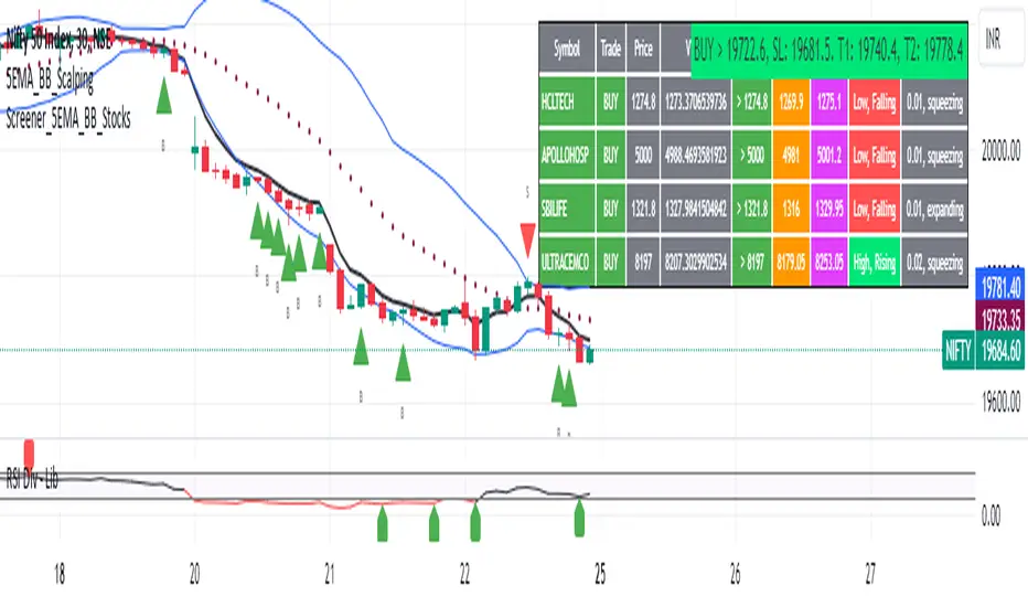
ROC (Rate of Change) Refurbished▮ Introduction
The Rate of Change indicator (ROC) is a momentum oscillator.
It was first introduced in the early 1970s by the American technical analyst Welles Wilder.
It calculates the percentage change in price between periods.
ROC takes the current price and compares it to a price 'n' periods (user defined) ago.
The calculated value is then plotted and fluctuates above and below a Zero Line.
A technical analyst may use ROC for:
- trend identification;
- identifying overbought and oversold conditions.
Even though ROC is an oscillator, it is not bounded to a set range.
The reason for this is that there is no limit to how far a security can advance in price but of course there is a limit to how far it can decline.
If price goes to $0, then it obviously will not decline any further.
Because of this, ROC can sometimes appear to be unbalanced.
(TradingView)
▮ Improvements
The following features were added:
1. Eight moving averages for the indicator;
2. Dynamic Zones;
3. Rules for coloring bars/candles.
▮ Motivation
Averages have been added to improve trend identification.
For finer tuning, you can choose the type of averages.
You can hide them if you don't need them.
The Dynamic Zones has been added to make it easier to identify overbought/oversold regions.
Unlike other oscillators like the RSI for example, the ROC does not have a predetermined range of oscillations.
Therefore, a fixed line that defines an overbought/oversold range becomes unfeasible.
It is in this matter that the Dynamic Zone helps.
It dynamically adjusts as the indicator oscillates.
▮ About Dynamic Zones
'Most indicators use a fixed zone for buy and sell signals.
Here's a concept based on zones that are responsive to the past levels of the indicator.'
The concept of Dynamic Zones was described by Leo Zamansky (Ph.D.) and David Stendahl, in the magazine of Stocks & Commodities V15:7 (306-310).
Basically, a statistical calculation is made to define the extreme levels, delimiting a possible overbought/oversold region.
Given user-defined probabilities, the percentile is calculated using the method of Nearest Rank.
It is calculated by taking the difference between the data point and the number of data points below it, then dividing by the total number of data points in the set.
The result is expressed as a percentage.
This provides a measure of how a particular value compares to other values in a data set, identifying outliers or values that are significantly higher or lower than the rest of the data.
▮ Thanks and Credits
- TradingView: for ROC and Moving Averages
- allanster: for Dynamic Zones

Price Correction to fix data manipulation and mispricingPrice Correction corrects for index and security mispricing to the extent possible in TradingView on both daily and intraday charts. Price correction addresses mispricing issues for specific securities with known issues, or the user can build daily candles from intraday data instead of relying on exchange reported daily OHLC prices, which can include both legitimate special auction and off-exchange trades or illegitimate mispricing. The user can also detect daily OHLC prices that don’t reflect the intraday price action within a specified percent deviation. Price Correction functions as normal candles or bars for any time frame when correction is not needed.
On the 4th of October 2022, the AMEX exchange, owned by the New York Stock Exchange, decided to misprice the daily OHLC data for the SPY, the world’s largest ETF fund. The exchange eliminated the overnight gap that should have occurred in the daily chart that represents regular trading hours by showing a wick connecting near the close of the previous day. Neither the SPX, the SP500 cash index that the SPY ETF tracks, nor other SPX ETFs such as VOO or IVV show such a wick because significant price action at that level never occurred. The intraday SPY chart never shows the price drop below 372.31 that day, but there is a wick that extends to 366.57. On the 6th of October, they continued this practice of using a wick that connects with the close of the previous day to eliminate gaps in daily price action. The objective of this indicator is to fix such inconsistent mispricing practices in the SPY, NYA, and other indices or securities.
Price Correction corrects for the daily mispricing in the SPY to agree with the price action that actually occurred in the SPX index it tracks, as well as the other SPX ETFs, by using intraday data. The chart below compares the Price Correction of the SPY (top) to the SPX (middle) and the original mispriced SPY (bottom) with incorrect wicks. Price correction (top) removes those incorrect wicks (bottom) to match the SPX (middle).
The daily mispricing of the SPY follows after the successful deployment of the NYSE Composite Index mispricing, NYA, an index that represents all common stocks within the New York Stock Exchange, the largest exchange in the world. The importance of the NYA should not be understated. It is the price counterpart to NYSE’s market internals or statistics. Beginning in 2021, the New York Stock Exchange eliminated gaps in daily OHLC data for the NYA by using the close of the previous day as the open for the following day, in violation of their own NYSE Index Series Methodology. The Methodology states for the opening price that “The first index level is calculated and published around 09:30 ET, when the U.S. equity markets open for their regular trading session. The calculation of that level utilizes the most updated prices available at that moment.” You can verify for yourself that this is simply not the case. The first update of the NYA price for each day matches the close of the previous day, not the “most updated prices available at that moment”, causing data providers to often represent the first intraday bar with a huge sudden price change when an overnight price change occurred instead. For example, on 13 Jun 2022, TradingView shows a one-minute bar drop 2.3%. With a market capitalization of roughly 23 trillion dollars, the NYSE composite capitalization did not suddenly drop a half-trillion dollars in just one minute as the intraday chart data would have you believe. All major US indices, index ETFs, and even foreign indices like the Toronto TAX, the Australian ASXAL, the Bombay SENSEX, and German DAX had down gaps that day, except for the mispriced NYSE index. Price Correction corrects for this mispricing in daily OHLC data, as shown in the main chart at the top of this page comparing the original NYA (top) to the Price Corrected NYA (bottom).
Price Correction also corrects for the intraday mispricing in the NYA. The chart below shows how the Price Correction (top) replaces the incorrect first one-minute candles with gaps (bottom) from 22 Sep 2022 to 29 Sep 2022. TradingView is inconsistent in how intraday data is reported for overnight gaps by sometimes connecting the first intraday bar of the day to the close of the previous day, and other times not. This inconsistency may be due to manually changing the intraday data based on user support tickets. For example, after reporting the lack of a major gap in the NYA daily OHLC prices that existed intraday for 13 Jun 2022, TradingView opted to remove the true gap in intraday prices by creating a 2.3% half-a-trillion-dollar one-minute bar that connected the close of the previous day to show a sudden drop in price that didn’t occur, instead of adding the gap in the daily OHLC data that actually took place from overnight price action.
Price Correction allows users to detect daily OHLC data that does not reflect the intraday price action within a certain percent difference by changing the color of those candles or bars that deviate. The chart below clearly shows the start of the NYSE disinformation campaign for NYA that started in 2021 by painting blue those candles with daily OHLC values that deviated from the intraday values by 0.1%. Before 2021, the number of deviating candles is relatively sparse, but beginning in 2021, the chart is littered with deviating candles.
If there are other index or security mispricing or data issues you are aware of that can be incorporated into Price Correction, please let me know. Accurate financial data is indispensable in making accurate financial decisions. Assert your right to accurate financial data by reporting incorrect data and mispricing issues.
How to use the Price Correction
Simply add this “indicator” to your chart and remove the mispriced default candles or bars by right clicking on the chart, selecting Settings, and de-selecting Body, Wick, and Border under the Symbol tab. The Presets settings automatically takes care of mispricing in the NYA and SPY to the extent possible in TradingView. The user can also build their own daily candles based off of intraday data to address other securities that may have mispricing issues.

MTF Stoch RSI + Realtime DivergencesMulti-timeframe Stochastic RSI + Realtime Divergences + Alerts + Pivot lookback periods.
This version of the Stochastic RSI adds the following additional features to the stock UO by Tradingview:
- Optional 3 x Multiple-timeframe overbought and oversold signals, indicating where 3 selected timeframes are all overbought (>80) or all oversold (<20) at the same time, with alert option.
- Optional divergence lines drawn directly onto the oscillator in realtime, with alert options.
- Configurable lookback periods to fine tune the divergences drawn in order to suit different trading styles and timeframes, including the ability to enable automatic adjustment of pivot period per chart timeframe.
- Alternate timeframe feature allows you to configure the oscillator to use data from a different timeframe than the chart it is loaded on.
- Indications where the Stoch RSI is crossing down from above the overbought threshold (<80) and crossing above the oversold threshold (>20) levels on a given user selected timeframe, by printing gold dots on the indicator.
- Also includes standard configurable Stoch RSI options, including k length, d length, RSI length, Stochastic length, and source type (close, hl2, etc)
While this version of the Stochastic RSI has the ability to draw divergences in realtime along with related settings and alerts so you can be notified as divergences occur without spending all day watching the charts, the main purpose of this indicator was to provide the triple multiple-timeframe overbought and oversold confluence signals and alerts, in an attempt to add more confluence, weight and reliability to the single timeframe overbought and oversold states, commonly used for trade entry confluence. It's primary purpose is intended for scalping on lower timeframes, typically between 1-15 minutes. The triple timeframe overbought can often indicate near term reversals to the downside, with the triple timeframe oversold often indicating neartime reversals to the upside. The default timeframes for this confluence are set to check the 1 minute, 5 minute, and 15 minute timeframes, ideal for scalping the < 15 minute charts.
The Stochastic RSI
The popular oscillator has been described as follows:
“The Stochastic RSI is an indicator used in technical analysis that ranges between zero and one (or zero and 100 on some charting platforms) and is created by applying the Stochastic oscillator formula to a set of relative strength index (RSI) values rather than to standard price data. Using RSI values within the Stochastic formula gives traders an idea of whether the current RSI value is overbought or oversold. The Stochastic RSI oscillator was developed to take advantage of both momentum indicators in order to create a more sensitive indicator that is attuned to a specific security's historical performance rather than a generalized analysis of price change.”
How do traders use overbought and oversold levels in their trading?
The oversold level, that is when the Stochastic RSI is above the 80 level is typically interpreted as being 'overbought', and below the 20 level is typically considered 'oversold'. Traders will often use the Stochastic RSI at an overbought level as a confluence for entry into a short position, and the Stochastic RSI at an oversold level as a confluence for an entry into a long position. These levels do not mean that price will necessarily reverse at those levels in a reliable way, however. This is why this version of the Stoch RSI employs the triple timeframe overbought and oversold confluence, in an attempt to add a more confluence and reliability to this usage of the Stoch RSI.
What are divergences?
Divergence is when the price of an asset is moving in the opposite direction of a technical indicator, such as an oscillator, or is moving contrary to other data. Divergence warns that the current price trend may be weakening, and in some cases may lead to the price changing direction.
There are 4 main types of divergence, which are split into 2 categories;
regular divergences and hidden divergences. Regular divergences indicate possible trend reversals, and hidden divergences indicate possible trend continuation.
Regular bullish divergence: An indication of a potential trend reversal, from the current downtrend, to an uptrend.
Regular bearish divergence: An indication of a potential trend reversal, from the current uptrend, to a downtrend.
Hidden bullish divergence: An indication of a potential uptrend continuation.
Hidden bearish divergence: An indication of a potential downtrend continuation.
Setting alerts.
With this indicator you can set alerts to notify you when any/all of the above types of divergences occur, on any chart timeframe you choose, and also when the triple timeframe overbought and oversold confluences occur.
Configurable pivot lookback values.
You can adjust the default pivot lookback values to suit your prefered trading style and timeframe. If you like to trade a shorter time frame, lowering the default lookback values will make the divergences drawn more sensitive to short term price action. By default, this indicator has enabled the automatic adjustment of the pivot periods for 4 configurable timeframes, in a bid to optimise the divergences drawn when the indicator is loaded onto any of the 4 timeframes. These timeframes and the auto adjusted pivot periods on each of them can also be reconfigured within the settings menu.
How do traders use divergences in their trading?
A divergence is considered a leading indicator in technical analysis , meaning it has the ability to indicate a potential price move in the short term future.
Hidden bullish and hidden bearish divergences, which indicate a potential continuation of the current trend are sometimes considered a good place for traders to begin, since trend continuation occurs more frequently than reversals, or trend changes.
When trading regular bullish divergences and regular bearish divergences, which are indications of a trend reversal, the probability of it doing so may increase when these occur at a strong support or resistance level . A common mistake new traders make is to get into a regular divergence trade too early, assuming it will immediately reverse, but these can continue to form for some time before the trend eventually changes, by using forms of support or resistance as an added confluence, such as when price reaches a moving average, the success rate when trading these patterns may increase.
Typically, traders will manually draw lines across the swing highs and swing lows of both the price chart and the oscillator to see whether they appear to present a divergence, this indicator will draw them for you, quickly and clearly, and can notify you when they occur.
Disclaimer: This script includes code from the stock UO by Tradingview as well as the Divergence for Many Indicators v4 by LonesomeTheBlue.

Crypto Portfolio ManagementCrypto Portfolio Management
This is an indicator not like the other ones that you regularly see in tradingview. The main difference is that this indicator does not plot a value for each candle bar like you would see with RSI or MACD. Actually it is table and it just uses tradingview great database of assets to plot some valuebale information that can not be found elsewhere easily. These metrics are some basic one that is used by portfolio managers to decide what they want to hold in their portfolio. The basic idea is that you should hold assets in your basket that are less correlated to the benchmark.
Benchmark in traditional context refers to main market indices like S&P 500 of US market. But they already have a lot of tools available. My effort was for crypto investors who are trying to rebalance their portfolio every month or week to have some good metrics to make decision. Because of this I used Bitcoin as crypto market benchmark. So, everything is compared to bitcoin in this script. I’m gonna explain the terms that is used in the table’s columns below.
MAKE SURE YOU PUT YOUR CHART AT DAILY AND AT THE MAXIMUM AVAILABLE DATA EXCHANGE.
Y-Exp
This is yearly expected return of the asset. It is simply the mean of the yearly returns of the asset. (these calculations are not typical in Tradingview because mainly we calculate on each bar and give value at the same bar but here this value to change once a year). Remember that the higher this value is the better it is because historically the asset have shown good returns but there is a tip: Always check the available historical data in any asset that you are adding if you add an asset that has only 1 year of data available or you use an exchange data that recently added the coin you will get unsignificant results and the results can not be trusted. You should always selects coins and market (coins can be changed in setting) that have the largest data available.
Y-SDev
This is a little bit complicated than the previous. This is the standard deviation of the yearly returns. This is a classic measure of RISK in financial markets. The higher the value, the more risk is involved with the asset that you have added. If you added two assets that have same returns but different Standard deviations, the rational thinker should choose the asset with lower Standard deviation.
The standard deviation is a good place to start but there are some considerations to have -it is getting complicated and average user should not be involved with these terms and can ignore the next phrases- standard deviation and mean of the yearly returns are random variables, these variables have a theoretical probability density function and these functions are not gaussian normal distribution. Because of this in the professional usage these returns should be transformed to a normal distribution and have all these terms calculated there and then transform back to its own normal state and then be used for any serious investment decision. I think these calculations can be done on Tradingview but I need you support to do this in the form of like and share of my scripts and ideas.
M-Exp and M-SDev
These terms are like the previous ones but it is calculated on monthly returns. As it goes for yearly return, the monthly returns change once a monthly candle closes. So be patient to use this indicator.
I highly recommend not to make decisions on monthly data due to a lot of noise involved with this market but in long run it is ok. So go with yearly returns and wait at least for 3 years to see your results.
CorToBTC
Basically you want to buy something that is less correalted with the benchmark. this is the correlation of the asset to bitcoin.
Sharpe Ratio
This is one of the most used metric as a risk adjusted return measurment. you can google it for more information. The higher this value the better. remmeber with any invenstment it is important to understand risks associated with the assets that you are buying.
DownFromATH
This metric that I didn't see anywhere in the tradingview and is familiar in the platforms like coinmarketcap. this is a real calculation of precentage down from ATH (All Time High). it means how much percentage a coin is down from the maximum price that the asset has experienced until now.
***
Remember you can change all the asset except main asset. If you like this script to 500 I will update this continuously.
