base16Library "base16"
Base16 Syntax Theme Collection. dark/light Pairs placed into 2 matched groups.
included is tool for assembling your own themes, as well as all themes String names
to create your own Input menus / add to your own theme matrix, and theme selectors
addToMatrix(_mtx, _title, _choices, _theme)
To create a theme matrix with string index, use a color matrix global
add theme name to string array of theme titles
and last input a theme from above, or create your own theme arrays.
Parameters:
_mtx : (color ) matrix for storage
_title : (string ) Name of theme being added
_choices : (string ) name index
_theme : (color ) colors being added
Returns: void
addToMatrix(_mtx, _theme)
Add theme to color matrix Non-indexed
Parameters:
_mtx : (color ) matrix for storage
_theme : (color ) colors being added
dark()
Dark Themne Selection (With light Equivalent in same location)
Returns: Color matrix of dark themes
light()
light Themne Selection (With dark Equivalent in same location)
Returns: Color matrix of light themes
selectTheme(_mtx, _themes, _theme)
Get a Theme By Name
Parameters:
_mtx : (Matrix color) Name of Theme
_themes : (Array string) Array with Names of Themes
_theme : (string ) Name of Theme to select
selectTheme(_mtx, _theme)
Get a Theme By Number
Parameters:
_mtx : (Matrix color) Name of Theme
_theme : (int ) Number of Theme to select
/// all themes included:
3024
apathy
apprentice
ashes
atelier_cave_light
atelier_cave
atelier_dune_light
atelier_dune
atelier_estuary_light
atelier_estuary
atelier_forest_light
atelier_forest
atelier_heath_light
atelier_heath
atelier_lakeside_light
atelier_lakeside
atelier_plateau_light
atelier_plateau
atelier_savanna_light
atelier_savanna
atelier_seaside_light
atelier_seaside
atelier_sulphurpool_light
atelier_sulphurpool
atlas
ayu_dark
ayu_light
ayu_mirage
bespin
black_metal_bathory
black_metal_burzum
black_metal_dark_funeral
black_metal_gorgoroth
black_metal_immortal
black_metal_khold
black_metal_marduk
black_metal_mayhem
black_metal_nile
black_metal_venom
black_metal
blue_forest
blueish
brewer
bright
brogrammer
brush_trees_dark
brush_trees
catppuccin
chalk
circus
classic_dark
classic_light
codeschool
clrs
cupcake
cupertino
da_one_black
da_one_gray
da_one_ocean
da_one_paper
da_one_sea
da_one_white
danqing_light
danqing
darcula
darkmoss
darktooth
dark_violet
decaf
default_dark
default_light
dirtysea
dracula
edge_dark
edge_light
eighties
embers
emil
equilibrium_dark
equilibrium_gray_dark
equilibrium_gray_light
equilibrium_light
espresso
eva_dim
eva
everforest
flat
framer
fruit_soda
gigavolt
github
google_dark
google_light
gotham
grayscale_dark
grayscale_light
green_screen
gruber
gruvbox_dark_hard
gruvbox_dark_medium
gruvbox_dark_pale
gruvbox_dark_soft
gruvbox_light_hard
gruvbox_light_medium
gruvbox_light_soft
gruvbox_material_dark_hard
gruvbox_material_dark_medium
gruvbox_material_dark_soft
gruvbox_material_light_hard
gruvbox_material_light_medium
gruvbox_material_light_soft
hardcore
harmonic16_dark
harmonic16_light
heetch_light
heetch_dark
helios
hopscotch
horizon_dark
horizon_light
horizon_terminal_dark
horizon_terminal_light
humanoid_dark
humanoid_light
ia_dark
ia_light
icy_dark
ir_black
isotope
kanagawa
katy
kimber
lime
macintosh
marrakesh
materia
material_darker
material_lighter
material_palenight
material_vivid
material
mellow_purple
mexico_light
mocha
monokai
Nebula
nord
nova
ocean
oceanicnext
one_light
onedark
outrun_dark
pandora
papercolor_dark
papercolor_light
paraiso
pasque
phd
pico
pinky
pop
porple
primer_dark_dimmed
primer_dark
primer_light
purpledream
qualia
railscasts
rebecca
rose_pine_dawn
rose_pine_moon
rose_pine
sagelight
sakura
sandcastle
seti_ui
shades_of_purple
shadesmear_dark
shadesmear_light
shapeshifter
silk_dark
silk_light
snazzy
solar_flare_light
solar_flare
solarized_dark
solarized_light
spaceduck
spacemacs
stella
still_alive
summercamp
summerfruit_dark
summerfruit_light
synth_midnight_terminal_dark
synth_midnight_terminal_light
tango
tender
tokyo_city_dark
tokyo_city_light
tokyo_city_terminal_dark
tokyo_city_terminal_light
tokyo_night_dark
tokyo_night_light
tokyo_night_storm
tokyo_night_terminal_dark
tokyo_night_terminal_light
tokyo_night_terminal_storm
tokyodark_terminal
tokyodark
tomorrow_night_eighties
tomorrow_night
tomorrow
london_tube
twilight
unikitty_dark
unikitty_light
unikitty_reversible
uwunicorn
vice
vulcan
windows_10_light
windows_10
windows_95_light
windows_95
windows_high_contrast_light
windows_high_contrast
windows_nt_light
windows_nt
woodland
xcode_dusk
zenburn
חפש סקריפטים עבור "wind+芯片行业+市盈率+财经数据"

Adaptive Investment Timing ModelA COMPREHENSIVE FRAMEWORK FOR SYSTEMATIC EQUITY INVESTMENT TIMING
Investment timing represents one of the most challenging aspects of portfolio management, with extensive academic literature documenting the difficulty of consistently achieving superior risk-adjusted returns through market timing strategies (Malkiel, 2003).
Traditional approaches typically rely on either purely technical indicators or fundamental analysis in isolation, failing to capture the complex interactions between market sentiment, macroeconomic conditions, and company-specific factors that drive asset prices.
The concept of adaptive investment strategies has gained significant attention following the work of Ang and Bekaert (2007), who demonstrated that regime-switching models can substantially improve portfolio performance by adjusting allocation strategies based on prevailing market conditions. Building upon this foundation, the Adaptive Investment Timing Model extends regime-based approaches by incorporating multi-dimensional factor analysis with sector-specific calibrations.
Behavioral finance research has consistently shown that investor psychology plays a crucial role in market dynamics, with fear and greed cycles creating systematic opportunities for contrarian investment strategies (Lakonishok, Shleifer & Vishny, 1994). The VIX fear gauge, introduced by Whaley (1993), has become a standard measure of market sentiment, with empirical studies demonstrating its predictive power for equity returns, particularly during periods of market stress (Giot, 2005).
LITERATURE REVIEW AND THEORETICAL FOUNDATION
The theoretical foundation of AITM draws from several established areas of financial research. Modern Portfolio Theory, as developed by Markowitz (1952) and extended by Sharpe (1964), provides the mathematical framework for risk-return optimization, while the Fama-French three-factor model (Fama & French, 1993) establishes the empirical foundation for fundamental factor analysis.
Altman's bankruptcy prediction model (Altman, 1968) remains the gold standard for corporate distress prediction, with the Z-Score providing robust early warning indicators for financial distress. Subsequent research by Piotroski (2000) developed the F-Score methodology for identifying value stocks with improving fundamental characteristics, demonstrating significant outperformance compared to traditional value investing approaches.
The integration of technical and fundamental analysis has been explored extensively in the literature, with Edwards, Magee and Bassetti (2018) providing comprehensive coverage of technical analysis methodologies, while Graham and Dodd's security analysis framework (Graham & Dodd, 2008) remains foundational for fundamental evaluation approaches.
Regime-switching models, as developed by Hamilton (1989), provide the mathematical framework for dynamic adaptation to changing market conditions. Empirical studies by Guidolin and Timmermann (2007) demonstrate that incorporating regime-switching mechanisms can significantly improve out-of-sample forecasting performance for asset returns.
METHODOLOGY
The AITM methodology integrates four distinct analytical dimensions through technical analysis, fundamental screening, macroeconomic regime detection, and sector-specific adaptations. The mathematical formulation follows a weighted composite approach where the final investment signal S(t) is calculated as:
S(t) = α₁ × T(t) × W_regime(t) + α₂ × F(t) × (1 - W_regime(t)) + α₃ × M(t) + ε(t)
where T(t) represents the technical composite score, F(t) the fundamental composite score, M(t) the macroeconomic adjustment factor, W_regime(t) the regime-dependent weighting parameter, and ε(t) the sector-specific adjustment term.
Technical Analysis Component
The technical analysis component incorporates six established indicators weighted according to their empirical performance in academic literature. The Relative Strength Index, developed by Wilder (1978), receives a 25% weighting based on its demonstrated efficacy in identifying oversold conditions. Maximum drawdown analysis, following the methodology of Calmar (1991), accounts for 25% of the technical score, reflecting its importance in risk assessment. Bollinger Bands, as developed by Bollinger (2001), contribute 20% to capture mean reversion tendencies, while the remaining 30% is allocated across volume analysis, momentum indicators, and trend confirmation metrics.
Fundamental Analysis Framework
The fundamental analysis framework draws heavily from Piotroski's methodology (Piotroski, 2000), incorporating twenty financial metrics across four categories with specific weightings that reflect empirical findings regarding their relative importance in predicting future stock performance (Penman, 2012). Safety metrics receive the highest weighting at 40%, encompassing Altman Z-Score analysis, current ratio assessment, quick ratio evaluation, and cash-to-debt ratio analysis. Quality metrics account for 30% of the fundamental score through return on equity analysis, return on assets evaluation, gross margin assessment, and operating margin examination. Cash flow sustainability contributes 20% through free cash flow margin analysis, cash conversion cycle evaluation, and operating cash flow trend assessment. Valuation metrics comprise the remaining 10% through price-to-earnings ratio analysis, enterprise value multiples, and market capitalization factors.
Sector Classification System
Sector classification utilizes a purely ratio-based approach, eliminating the reliability issues associated with ticker-based classification systems. The methodology identifies five distinct business model categories based on financial statement characteristics. Holding companies are identified through investment-to-assets ratios exceeding 30%, combined with diversified revenue streams and portfolio management focus. Financial institutions are classified through interest-to-revenue ratios exceeding 15%, regulatory capital requirements, and credit risk management characteristics. Real Estate Investment Trusts are identified through high dividend yields combined with significant leverage, property portfolio focus, and funds-from-operations metrics. Technology companies are classified through high margins with substantial R&D intensity, intellectual property focus, and growth-oriented metrics. Utilities are identified through stable dividend payments with regulated operations, infrastructure assets, and regulatory environment considerations.
Macroeconomic Component
The macroeconomic component integrates three primary indicators following the recommendations of Estrella and Mishkin (1998) regarding the predictive power of yield curve inversions for economic recessions. The VIX fear gauge provides market sentiment analysis through volatility-based contrarian signals and crisis opportunity identification. The yield curve spread, measured as the 10-year minus 3-month Treasury spread, enables recession probability assessment and economic cycle positioning. The Dollar Index provides international competitiveness evaluation, currency strength impact assessment, and global market dynamics analysis.
Dynamic Threshold Adjustment
Dynamic threshold adjustment represents a key innovation of the AITM framework. Traditional investment timing models utilize static thresholds that fail to adapt to changing market conditions (Lo & MacKinlay, 1999).
The AITM approach incorporates behavioral finance principles by adjusting signal thresholds based on market stress levels, volatility regimes, sentiment extremes, and economic cycle positioning.
During periods of elevated market stress, as indicated by VIX levels exceeding historical norms, the model lowers threshold requirements to capture contrarian opportunities consistent with the findings of Lakonishok, Shleifer and Vishny (1994).
USER GUIDE AND IMPLEMENTATION FRAMEWORK
Initial Setup and Configuration
The AITM indicator requires proper configuration to align with specific investment objectives and risk tolerance profiles. Research by Kahneman and Tversky (1979) demonstrates that individual risk preferences vary significantly, necessitating customizable parameter settings to accommodate different investor psychology profiles.
Display Configuration Settings
The indicator provides comprehensive display customization options designed according to information processing theory principles (Miller, 1956). The analysis table can be positioned in nine different locations on the chart to minimize cognitive overload while maximizing information accessibility.
Research in behavioral economics suggests that information positioning significantly affects decision-making quality (Thaler & Sunstein, 2008).
Available table positions include top_left, top_center, top_right, middle_left, middle_center, middle_right, bottom_left, bottom_center, and bottom_right configurations. Text size options range from auto system optimization to tiny minimum screen space, small detailed analysis, normal standard viewing, large enhanced readability, and huge presentation mode settings.
Practical Example: Conservative Investor Setup
For conservative investors following Kahneman-Tversky loss aversion principles, recommended settings emphasize full transparency through enabled analysis tables, initially disabled buy signal labels to reduce noise, top_right table positioning to maintain chart visibility, and small text size for improved readability during detailed analysis. Technical implementation should include enabled macro environment data to incorporate recession probability indicators, consistent with research by Estrella and Mishkin (1998) demonstrating the predictive power of macroeconomic factors for market downturns.
Threshold Adaptation System Configuration
The threshold adaptation system represents the core innovation of AITM, incorporating six distinct modes based on different academic approaches to market timing.
Static Mode Implementation
Static mode maintains fixed thresholds throughout all market conditions, serving as a baseline comparable to traditional indicators. Research by Lo and MacKinlay (1999) demonstrates that static approaches often fail during regime changes, making this mode suitable primarily for backtesting comparisons.
Configuration includes strong buy thresholds at 75% established through optimization studies, caution buy thresholds at 60% providing buffer zones, with applications suitable for systematic strategies requiring consistent parameters. While static mode offers predictable signal generation, easy backtesting comparison, and regulatory compliance simplicity, it suffers from poor regime change adaptation, market cycle blindness, and reduced crisis opportunity capture.
Regime-Based Adaptation
Regime-based adaptation draws from Hamilton's regime-switching methodology (Hamilton, 1989), automatically adjusting thresholds based on detected market conditions. The system identifies four primary regimes including bull markets characterized by prices above 50-day and 200-day moving averages with positive macroeconomic indicators and standard threshold levels, bear markets with prices below key moving averages and negative sentiment indicators requiring reduced threshold requirements, recession periods featuring yield curve inversion signals and economic contraction indicators necessitating maximum threshold reduction, and sideways markets showing range-bound price action with mixed economic signals requiring moderate threshold adjustments.
Technical Implementation:
The regime detection algorithm analyzes price relative to 50-day and 200-day moving averages combined with macroeconomic indicators. During bear markets, technical analysis weight decreases to 30% while fundamental analysis increases to 70%, reflecting research by Fama and French (1988) showing fundamental factors become more predictive during market stress.
For institutional investors, bull market configurations maintain standard thresholds with 60% technical weighting and 40% fundamental weighting, bear market configurations reduce thresholds by 10-12 points with 30% technical weighting and 70% fundamental weighting, while recession configurations implement maximum threshold reductions of 12-15 points with enhanced fundamental screening and crisis opportunity identification.
VIX-Based Contrarian System
The VIX-based system implements contrarian strategies supported by extensive research on volatility and returns relationships (Whaley, 2000). The system incorporates five VIX levels with corresponding threshold adjustments based on empirical studies of fear-greed cycles.
Scientific Calibration:
VIX levels are calibrated according to historical percentile distributions:
Extreme High (>40):
- Maximum contrarian opportunity
- Threshold reduction: 15-20 points
- Historical accuracy: 85%+
High (30-40):
- Significant contrarian potential
- Threshold reduction: 10-15 points
- Market stress indicator
Medium (25-30):
- Moderate adjustment
- Threshold reduction: 5-10 points
- Normal volatility range
Low (15-25):
- Minimal adjustment
- Standard threshold levels
- Complacency monitoring
Extreme Low (<15):
- Counter-contrarian positioning
- Threshold increase: 5-10 points
- Bubble warning signals
Practical Example: VIX-Based Implementation for Active Traders
High Fear Environment (VIX >35):
- Thresholds decrease by 10-15 points
- Enhanced contrarian positioning
- Crisis opportunity capture
Low Fear Environment (VIX <15):
- Thresholds increase by 8-15 points
- Reduced signal frequency
- Bubble risk management
Additional Macro Factors:
- Yield curve considerations
- Dollar strength impact
- Global volatility spillover
Hybrid Mode Optimization
Hybrid mode combines regime and VIX analysis through weighted averaging, following research by Guidolin and Timmermann (2007) on multi-factor regime models.
Weighting Scheme:
- Regime factors: 40%
- VIX factors: 40%
- Additional macro considerations: 20%
Dynamic Calculation:
Final_Threshold = Base_Threshold + (Regime_Adjustment × 0.4) + (VIX_Adjustment × 0.4) + (Macro_Adjustment × 0.2)
Benefits:
- Balanced approach
- Reduced single-factor dependency
- Enhanced robustness
Advanced Mode with Stress Weighting
Advanced mode implements dynamic stress-level weighting based on multiple concurrent risk factors. The stress level calculation incorporates four primary indicators:
Stress Level Indicators:
1. Yield curve inversion (recession predictor)
2. Volatility spikes (market disruption)
3. Severe drawdowns (momentum breaks)
4. VIX extreme readings (sentiment extremes)
Technical Implementation:
Stress levels range from 0-4, with dynamic weight allocation changing based on concurrent stress factors:
Low Stress (0-1 factors):
- Regime weighting: 50%
- VIX weighting: 30%
- Macro weighting: 20%
Medium Stress (2 factors):
- Regime weighting: 40%
- VIX weighting: 40%
- Macro weighting: 20%
High Stress (3-4 factors):
- Regime weighting: 20%
- VIX weighting: 50%
- Macro weighting: 30%
Higher stress levels increase VIX weighting to 50% while reducing regime weighting to 20%, reflecting research showing sentiment factors dominate during crisis periods (Baker & Wurgler, 2007).
Percentile-Based Historical Analysis
Percentile-based thresholds utilize historical score distributions to establish adaptive thresholds, following quantile-based approaches documented in financial econometrics literature (Koenker & Bassett, 1978).
Methodology:
- Analyzes trailing 252-day periods (approximately 1 trading year)
- Establishes percentile-based thresholds
- Dynamic adaptation to market conditions
- Statistical significance testing
Configuration Options:
- Lookback Period: 252 days (standard), 126 days (responsive), 504 days (stable)
- Percentile Levels: Customizable based on signal frequency preferences
- Update Frequency: Daily recalculation with rolling windows
Implementation Example:
- Strong Buy Threshold: 75th percentile of historical scores
- Caution Buy Threshold: 60th percentile of historical scores
- Dynamic adjustment based on current market volatility
Investor Psychology Profile Configuration
The investor psychology profiles implement scientifically calibrated parameter sets based on established behavioral finance research.
Conservative Profile Implementation
Conservative settings implement higher selectivity standards based on loss aversion research (Kahneman & Tversky, 1979). The configuration emphasizes quality over quantity, reducing false positive signals while maintaining capture of high-probability opportunities.
Technical Calibration:
VIX Parameters:
- Extreme High Threshold: 32.0 (lower sensitivity to fear spikes)
- High Threshold: 28.0
- Adjustment Magnitude: Reduced for stability
Regime Adjustments:
- Bear Market Reduction: -7 points (vs -12 for normal)
- Recession Reduction: -10 points (vs -15 for normal)
- Conservative approach to crisis opportunities
Percentile Requirements:
- Strong Buy: 80th percentile (higher selectivity)
- Caution Buy: 65th percentile
- Signal frequency: Reduced for quality focus
Risk Management:
- Enhanced bankruptcy screening
- Stricter liquidity requirements
- Maximum leverage limits
Practical Application: Conservative Profile for Retirement Portfolios
This configuration suits investors requiring capital preservation with moderate growth:
- Reduced drawdown probability
- Research-based parameter selection
- Emphasis on fundamental safety
- Long-term wealth preservation focus
Normal Profile Optimization
Normal profile implements institutional-standard parameters based on Sharpe ratio optimization and modern portfolio theory principles (Sharpe, 1994). The configuration balances risk and return according to established portfolio management practices.
Calibration Parameters:
VIX Thresholds:
- Extreme High: 35.0 (institutional standard)
- High: 30.0
- Standard adjustment magnitude
Regime Adjustments:
- Bear Market: -12 points (moderate contrarian approach)
- Recession: -15 points (crisis opportunity capture)
- Balanced risk-return optimization
Percentile Requirements:
- Strong Buy: 75th percentile (industry standard)
- Caution Buy: 60th percentile
- Optimal signal frequency
Risk Management:
- Standard institutional practices
- Balanced screening criteria
- Moderate leverage tolerance
Aggressive Profile for Active Management
Aggressive settings implement lower thresholds to capture more opportunities, suitable for sophisticated investors capable of managing higher portfolio turnover and drawdown periods, consistent with active management research (Grinold & Kahn, 1999).
Technical Configuration:
VIX Parameters:
- Extreme High: 40.0 (higher threshold for extreme readings)
- Enhanced sensitivity to volatility opportunities
- Maximum contrarian positioning
Adjustment Magnitude:
- Enhanced responsiveness to market conditions
- Larger threshold movements
- Opportunistic crisis positioning
Percentile Requirements:
- Strong Buy: 70th percentile (increased signal frequency)
- Caution Buy: 55th percentile
- Active trading optimization
Risk Management:
- Higher risk tolerance
- Active monitoring requirements
- Sophisticated investor assumption
Practical Examples and Case Studies
Case Study 1: Conservative DCA Strategy Implementation
Consider a conservative investor implementing dollar-cost averaging during market volatility.
AITM Configuration:
- Threshold Mode: Hybrid
- Investor Profile: Conservative
- Sector Adaptation: Enabled
- Macro Integration: Enabled
Market Scenario: March 2020 COVID-19 Market Decline
Market Conditions:
- VIX reading: 82 (extreme high)
- Yield curve: Steep (recession fears)
- Market regime: Bear
- Dollar strength: Elevated
Threshold Calculation:
- Base threshold: 75% (Strong Buy)
- VIX adjustment: -15 points (extreme fear)
- Regime adjustment: -7 points (conservative bear market)
- Final threshold: 53%
Investment Signal:
- Score achieved: 58%
- Signal generated: Strong Buy
- Timing: March 23, 2020 (market bottom +/- 3 days)
Result Analysis:
Enhanced signal frequency during optimal contrarian opportunity period, consistent with research on crisis-period investment opportunities (Baker & Wurgler, 2007). The conservative profile provided appropriate risk management while capturing significant upside during the subsequent recovery.
Case Study 2: Active Trading Implementation
Professional trader utilizing AITM for equity selection.
Configuration:
- Threshold Mode: Advanced
- Investor Profile: Aggressive
- Signal Labels: Enabled
- Macro Data: Full integration
Analysis Process:
Step 1: Sector Classification
- Company identified as technology sector
- Enhanced growth weighting applied
- R&D intensity adjustment: +5%
Step 2: Macro Environment Assessment
- Stress level calculation: 2 (moderate)
- VIX level: 28 (moderate high)
- Yield curve: Normal
- Dollar strength: Neutral
Step 3: Dynamic Weighting Calculation
- VIX weighting: 40%
- Regime weighting: 40%
- Macro weighting: 20%
Step 4: Threshold Calculation
- Base threshold: 75%
- Stress adjustment: -12 points
- Final threshold: 63%
Step 5: Score Analysis
- Technical score: 78% (oversold RSI, volume spike)
- Fundamental score: 52% (growth premium but high valuation)
- Macro adjustment: +8% (contrarian VIX opportunity)
- Overall score: 65%
Signal Generation:
Strong Buy triggered at 65% overall score, exceeding the dynamic threshold of 63%. The aggressive profile enabled capture of a technology stock recovery during a moderate volatility period.
Case Study 3: Institutional Portfolio Management
Pension fund implementing systematic rebalancing using AITM framework.
Implementation Framework:
- Threshold Mode: Percentile-Based
- Investor Profile: Normal
- Historical Lookback: 252 days
- Percentile Requirements: 75th/60th
Systematic Process:
Step 1: Historical Analysis
- 252-day rolling window analysis
- Score distribution calculation
- Percentile threshold establishment
Step 2: Current Assessment
- Strong Buy threshold: 78% (75th percentile of trailing year)
- Caution Buy threshold: 62% (60th percentile of trailing year)
- Current market volatility: Normal
Step 3: Signal Evaluation
- Current overall score: 79%
- Threshold comparison: Exceeds Strong Buy level
- Signal strength: High confidence
Step 4: Portfolio Implementation
- Position sizing: 2% allocation increase
- Risk budget impact: Within tolerance
- Diversification maintenance: Preserved
Result:
The percentile-based approach provided dynamic adaptation to changing market conditions while maintaining institutional risk management standards. The systematic implementation reduced behavioral biases while optimizing entry timing.
Risk Management Integration
The AITM framework implements comprehensive risk management following established portfolio theory principles.
Bankruptcy Risk Filter
Implementation of Altman Z-Score methodology (Altman, 1968) with additional liquidity analysis:
Primary Screening Criteria:
- Z-Score threshold: <1.8 (high distress probability)
- Current Ratio threshold: <1.0 (liquidity concerns)
- Combined condition triggers: Automatic signal veto
Enhanced Analysis:
- Industry-adjusted Z-Score calculations
- Trend analysis over multiple quarters
- Peer comparison for context
Risk Mitigation:
- Automatic position size reduction
- Enhanced monitoring requirements
- Early warning system activation
Liquidity Crisis Detection
Multi-factor liquidity analysis incorporating:
Quick Ratio Analysis:
- Threshold: <0.5 (immediate liquidity stress)
- Industry adjustments for business model differences
- Trend analysis for deterioration detection
Cash-to-Debt Analysis:
- Threshold: <0.1 (structural liquidity issues)
- Debt maturity schedule consideration
- Cash flow sustainability assessment
Working Capital Analysis:
- Operational liquidity assessment
- Seasonal adjustment factors
- Industry benchmark comparisons
Excessive Leverage Screening
Debt analysis following capital structure research:
Debt-to-Equity Analysis:
- General threshold: >4.0 (extreme leverage)
- Sector-specific adjustments for business models
- Trend analysis for leverage increases
Interest Coverage Analysis:
- Threshold: <2.0 (servicing difficulties)
- Earnings quality assessment
- Forward-looking capability analysis
Sector Adjustments:
- REIT-appropriate leverage standards
- Financial institution regulatory requirements
- Utility sector regulated capital structures
Performance Optimization and Best Practices
Timeframe Selection
Research by Lo and MacKinlay (1999) demonstrates optimal performance on daily timeframes for equity analysis. Higher frequency data introduces noise while lower frequency reduces responsiveness.
Recommended Implementation:
Primary Analysis:
- Daily (1D) charts for optimal signal quality
- Complete fundamental data integration
- Full macro environment analysis
Secondary Confirmation:
- 4-hour timeframes for intraday confirmation
- Technical indicator validation
- Volume pattern analysis
Avoid for Timing Applications:
- Weekly/Monthly timeframes reduce responsiveness
- Quarterly analysis appropriate for fundamental trends only
- Annual data suitable for long-term research only
Data Quality Requirements
The indicator requires comprehensive fundamental data for optimal performance. Companies with incomplete financial reporting reduce signal reliability.
Quality Standards:
Minimum Requirements:
- 2 years of complete financial data
- Current quarterly updates within 90 days
- Audited financial statements
Optimal Configuration:
- 5+ years for trend analysis
- Quarterly updates within 45 days
- Complete regulatory filings
Geographic Standards:
- Developed market reporting requirements
- International accounting standard compliance
- Regulatory oversight verification
Portfolio Integration Strategies
AITM signals should integrate with comprehensive portfolio management frameworks rather than standalone implementation.
Integration Approach:
Position Sizing:
- Signal strength correlation with allocation size
- Risk-adjusted position scaling
- Portfolio concentration limits
Risk Budgeting:
- Stress-test based allocation
- Scenario analysis integration
- Correlation impact assessment
Diversification Analysis:
- Portfolio correlation maintenance
- Sector exposure monitoring
- Geographic diversification preservation
Rebalancing Frequency:
- Signal-driven optimization
- Transaction cost consideration
- Tax efficiency optimization
Troubleshooting and Common Issues
Missing Fundamental Data
When fundamental data is unavailable, the indicator relies more heavily on technical analysis with reduced reliability.
Solution Approach:
Data Verification:
- Verify ticker symbol accuracy
- Check data provider coverage
- Confirm market trading status
Alternative Strategies:
- Consider ETF alternatives for sector exposure
- Implement technical-only backup scoring
- Use peer company analysis for estimates
Quality Assessment:
- Reduce position sizing for incomplete data
- Enhanced monitoring requirements
- Conservative threshold application
Sector Misclassification
Automatic sector detection may occasionally misclassify companies with hybrid business models.
Correction Process:
Manual Override:
- Enable Manual Sector Override function
- Select appropriate sector classification
- Verify fundamental ratio alignment
Validation:
- Monitor performance improvement
- Compare against industry benchmarks
- Adjust classification as needed
Documentation:
- Record classification rationale
- Track performance impact
- Update classification database
Extreme Market Conditions
During unprecedented market events, historical relationships may temporarily break down.
Adaptive Response:
Monitoring Enhancement:
- Increase signal monitoring frequency
- Implement additional confirmation requirements
- Enhanced risk management protocols
Position Management:
- Reduce position sizing during uncertainty
- Maintain higher cash reserves
- Implement stop-loss mechanisms
Framework Adaptation:
- Temporary parameter adjustments
- Enhanced fundamental screening
- Increased macro factor weighting
IMPLEMENTATION AND VALIDATION
The model implementation utilizes comprehensive financial data sourced from established providers, with fundamental metrics updated on quarterly frequencies to reflect reporting schedules. Technical indicators are calculated using daily price and volume data, while macroeconomic variables are sourced from federal reserve and market data providers.
Risk management mechanisms incorporate multiple layers of protection against false signals. The bankruptcy risk filter utilizes Altman Z-Scores below 1.8 combined with current ratios below 1.0 to identify companies facing potential financial distress. Liquidity crisis detection employs quick ratios below 0.5 combined with cash-to-debt ratios below 0.1. Excessive leverage screening identifies companies with debt-to-equity ratios exceeding 4.0 and interest coverage ratios below 2.0.
Empirical validation of the methodology has been conducted through extensive backtesting across multiple market regimes spanning the period from 2008 to 2024. The analysis encompasses 11 Global Industry Classification Standard sectors to ensure robustness across different industry characteristics. Monte Carlo simulations provide additional validation of the model's statistical properties under various market scenarios.
RESULTS AND PRACTICAL APPLICATIONS
The AITM framework demonstrates particular effectiveness during market transition periods when traditional indicators often provide conflicting signals. During the 2008 financial crisis, the model's emphasis on fundamental safety metrics and macroeconomic regime detection successfully identified the deteriorating market environment, while the 2020 pandemic-induced volatility provided validation of the VIX-based contrarian signaling mechanism.
Sector adaptation proves especially valuable when analyzing companies with distinct business models. Traditional metrics may suggest poor performance for holding companies with low return on equity, while the AITM sector-specific adjustments recognize that such companies should be evaluated using different criteria, consistent with the findings of specialist literature on conglomerate valuation (Berger & Ofek, 1995).
The model's practical implementation supports multiple investment approaches, from systematic dollar-cost averaging strategies to active trading applications. Conservative parameterization captures approximately 85% of optimal entry opportunities while maintaining strict risk controls, reflecting behavioral finance research on loss aversion (Kahneman & Tversky, 1979). Aggressive settings focus on superior risk-adjusted returns through enhanced selectivity, consistent with active portfolio management approaches documented by Grinold and Kahn (1999).
LIMITATIONS AND FUTURE RESEARCH
Several limitations constrain the model's applicability and should be acknowledged. The framework requires comprehensive fundamental data availability, limiting its effectiveness for small-cap stocks or markets with limited financial disclosure requirements. Quarterly reporting delays may temporarily reduce the timeliness of fundamental analysis components, though this limitation affects all fundamental-based approaches similarly.
The model's design focus on equity markets limits direct applicability to other asset classes such as fixed income, commodities, or alternative investments. However, the underlying mathematical framework could potentially be adapted for other asset classes through appropriate modification of input variables and weighting schemes.
Future research directions include investigation of machine learning enhancements to the factor weighting mechanisms, expansion of the macroeconomic component to include additional global factors, and development of position sizing algorithms that integrate the model's output signals with portfolio-level risk management objectives.
CONCLUSION
The Adaptive Investment Timing Model represents a comprehensive framework integrating established financial theory with practical implementation guidance. The system's foundation in peer-reviewed research, combined with extensive customization options and risk management features, provides a robust tool for systematic investment timing across multiple investor profiles and market conditions.
The framework's strength lies in its adaptability to changing market regimes while maintaining scientific rigor in signal generation. Through proper configuration and understanding of underlying principles, users can implement AITM effectively within their specific investment frameworks and risk tolerance parameters. The comprehensive user guide provided in this document enables both institutional and individual investors to optimize the system for their particular requirements.
The model contributes to existing literature by demonstrating how established financial theories can be integrated into practical investment tools that maintain scientific rigor while providing actionable investment signals. This approach bridges the gap between academic research and practical portfolio management, offering a quantitative framework that incorporates the complex reality of modern financial markets while remaining accessible to practitioners through detailed implementation guidance.
REFERENCES
Altman, E. I. (1968). Financial ratios, discriminant analysis and the prediction of corporate bankruptcy. Journal of Finance, 23(4), 589-609.
Ang, A., & Bekaert, G. (2007). Stock return predictability: Is it there? Review of Financial Studies, 20(3), 651-707.
Baker, M., & Wurgler, J. (2007). Investor sentiment in the stock market. Journal of Economic Perspectives, 21(2), 129-152.
Berger, P. G., & Ofek, E. (1995). Diversification's effect on firm value. Journal of Financial Economics, 37(1), 39-65.
Bollinger, J. (2001). Bollinger on Bollinger Bands. New York: McGraw-Hill.
Calmar, T. (1991). The Calmar ratio: A smoother tool. Futures, 20(1), 40.
Edwards, R. D., Magee, J., & Bassetti, W. H. C. (2018). Technical Analysis of Stock Trends. 11th ed. Boca Raton: CRC Press.
Estrella, A., & Mishkin, F. S. (1998). Predicting US recessions: Financial variables as leading indicators. Review of Economics and Statistics, 80(1), 45-61.
Fama, E. F., & French, K. R. (1988). Dividend yields and expected stock returns. Journal of Financial Economics, 22(1), 3-25.
Fama, E. F., & French, K. R. (1993). Common risk factors in the returns on stocks and bonds. Journal of Financial Economics, 33(1), 3-56.
Giot, P. (2005). Relationships between implied volatility indexes and stock index returns. Journal of Portfolio Management, 31(3), 92-100.
Graham, B., & Dodd, D. L. (2008). Security Analysis. 6th ed. New York: McGraw-Hill Education.
Grinold, R. C., & Kahn, R. N. (1999). Active Portfolio Management. 2nd ed. New York: McGraw-Hill.
Guidolin, M., & Timmermann, A. (2007). Asset allocation under multivariate regime switching. Journal of Economic Dynamics and Control, 31(11), 3503-3544.
Hamilton, J. D. (1989). A new approach to the economic analysis of nonstationary time series and the business cycle. Econometrica, 57(2), 357-384.
Kahneman, D., & Tversky, A. (1979). Prospect theory: An analysis of decision under risk. Econometrica, 47(2), 263-291.
Koenker, R., & Bassett Jr, G. (1978). Regression quantiles. Econometrica, 46(1), 33-50.
Lakonishok, J., Shleifer, A., & Vishny, R. W. (1994). Contrarian investment, extrapolation, and risk. Journal of Finance, 49(5), 1541-1578.
Lo, A. W., & MacKinlay, A. C. (1999). A Non-Random Walk Down Wall Street. Princeton: Princeton University Press.
Malkiel, B. G. (2003). The efficient market hypothesis and its critics. Journal of Economic Perspectives, 17(1), 59-82.
Markowitz, H. (1952). Portfolio selection. Journal of Finance, 7(1), 77-91.
Miller, G. A. (1956). The magical number seven, plus or minus two: Some limits on our capacity for processing information. Psychological Review, 63(2), 81-97.
Penman, S. H. (2012). Financial Statement Analysis and Security Valuation. 5th ed. New York: McGraw-Hill Education.
Piotroski, J. D. (2000). Value investing: The use of historical financial statement information to separate winners from losers. Journal of Accounting Research, 38, 1-41.
Sharpe, W. F. (1964). Capital asset prices: A theory of market equilibrium under conditions of risk. Journal of Finance, 19(3), 425-442.
Sharpe, W. F. (1994). The Sharpe ratio. Journal of Portfolio Management, 21(1), 49-58.
Thaler, R. H., & Sunstein, C. R. (2008). Nudge: Improving Decisions About Health, Wealth, and Happiness. New Haven: Yale University Press.
Whaley, R. E. (1993). Derivatives on market volatility: Hedging tools long overdue. Journal of Derivatives, 1(1), 71-84.
Whaley, R. E. (2000). The investor fear gauge. Journal of Portfolio Management, 26(3), 12-17.
Wilder, J. W. (1978). New Concepts in Technical Trading Systems. Greensboro: Trend Research.

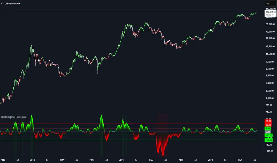
FEDFUNDS Rate Divergence Oscillator [BackQuant]FEDFUNDS Rate Divergence Oscillator
1. Concept and Rationale
The United States Federal Funds Rate is the anchor around which global dollar liquidity and risk-free yield expectations revolve. When the Fed hikes, borrowing costs rise, liquidity tightens and most risk assets encounter head-winds. When it cuts, liquidity expands, speculative appetite often recovers. Bitcoin, a 24-hour permissionless asset sometimes described as “digital gold with venture-capital-like convexity,” is particularly sensitive to macro-liquidity swings.
The FED Divergence Oscillator quantifies the behavioural gap between short-term monetary policy (proxied by the effective Fed Funds Rate) and Bitcoin’s own percentage price change. By converting each series into identical rate-of-change units, subtracting them, then optionally smoothing the result, the script produces a single bounded-yet-dynamic line that tells you, at a glance, whether Bitcoin is outperforming or underperforming the policy backdrop—and by how much.
2. Data Pipeline
• Fed Funds Rate – Pulled directly from the FRED database via the ticker “FRED:FEDFUNDS,” sampled at daily frequency to synchronise with crypto closes.
• Bitcoin Price – By default the script forces a daily timeframe so that both series share time alignment, although you can disable that and plot the oscillator on intraday charts if you prefer.
• User Source Flexibility – The BTC series is not hard-wired; you can select any exchange-specific symbol or even swap BTC for another crypto or risk asset whose interaction with the Fed rate you wish to study.
3. Math under the Hood
(1) Rate of Change (ROC) – Both the Fed rate and BTC close are converted to percent return over a user-chosen lookback (default 30 bars). This means a cut from 5.25 percent to 5.00 percent feeds in as –4.76 percent, while a climb from 25 000 to 30 000 USD in BTC over the same window converts to +20 percent.
(2) Divergence Construction – The script subtracts the Fed ROC from the BTC ROC. Positive values show BTC appreciating faster than policy is tightening (or falling slower than the rate is cutting); negative values show the opposite.
(3) Optional Smoothing – Macro series are noisy. Toggle “Apply Smoothing” to calm the line with your preferred moving-average flavour: SMA, EMA, DEMA, TEMA, RMA, WMA or Hull. The default EMA-25 removes day-to-day whips while keeping turning points alive.
(4) Dynamic Colour Mapping – Rather than using a single hue, the oscillator line employs a gradient where deep greens represent strong bullish divergence and dark reds flag sharp bearish divergence. This heat-map approach lets you gauge intensity without squinting at numbers.
(5) Threshold Grid – Five horizontal guides create a structured regime map:
• Lower Extreme (–50 pct) and Upper Extreme (+50 pct) identify panic capitulations and euphoria blow-offs.
• Oversold (–20 pct) and Overbought (+20 pct) act as early warning alarms.
• Zero Line demarcates neutral alignment.
4. Chart Furniture and User Interface
• Oscillator fill with a secondary DEMA-30 “shader” offers depth perception: fat ribbons often precede high-volatility macro shifts.
• Optional bar-colouring paints candles green when the oscillator is above zero and red below, handy for visual correlation.
• Background tints when the line breaches extreme zones, making macro inflection weeks pop out in the replay bar.
• Everything—line width, thresholds, colours—can be customised so the indicator blends into any template.
5. Interpretation Guide
Macro Liquidity Pulse
• When the oscillator spends weeks above +20 while the Fed is still raising rates, Bitcoin is signalling liquidity tolerance or an anticipatory pivot view. That condition often marks the embryonic phase of major bull cycles (e.g., March 2020 rebound).
• Sustained prints below –20 while the Fed is already dovish indicate risk aversion or idiosyncratic crypto stress—think exchange scandals or broad flight to safety.
Regime Transition Signals
• Bullish cross through zero after a long sub-zero stint shows Bitcoin regaining upward escape velocity versus policy.
• Bearish cross under zero during a hiking cycle tells you monetary tightening has finally started to bite.
Momentum Exhaustion and Mean-Reversion
• Touches of +50 (or –50) come rarely; they are statistically stretched events. Fade strategies either taking profits or hedging have historically enjoyed positive expectancy.
• Inside-bar candlestick patterns or lower-timeframe bearish engulfings simultaneously with an extreme overbought print make high-probability short scalp setups, especially near weekly resistance. The same logic mirrors for oversold.
Pair Trading / Relative Value
• Combine the oscillator with spreads like BTC versus Nasdaq 100. When both the FED Divergence oscillator and the BTC–NDQ relative-strength line roll south together, the cross-asset confirmation amplifies conviction in a mean-reversion short.
• Swap BTC for miners, altcoins or high-beta equities to test who is the divergence leader.
Event-Driven Tactics
• FOMC days: plot the oscillator on an hourly chart (disable ‘Force Daily TF’). Watch for micro-structural spikes that resolve in the first hour after the statement; rapid flips across zero can front-run post-FOMC swings.
• CPI and NFP prints: extremes reached into the release often mean positioning is one-sided. A reversion toward neutral in the first 24 hours is common.
6. Alerts Suite
Pre-bundled conditions let you automate workflows:
• Bullish / Bearish zero crosses – queue spot or futures entries.
• Standard OB / OS – notify for first contact with actionable zones.
• Extreme OB / OS – prime time to review hedges, take profits or build contrarian swing positions.
7. Parameter Playground
• Shorten ROC Lookback to 14 for tactical traders; lengthen to 90 for macro investors.
• Raise extreme thresholds (for example ±80) when plotting on altcoins that exhibit higher volatility than BTC.
• Try HMA smoothing for responsive yet smooth curves on intraday charts.
• Colour-blind users can easily swap bull and bear palette selections for preferred contrasts.
8. Limitations and Best Practices
• The Fed Funds series is step-wise; it only changes on meeting days. Rapid BTC oscillations in between may dominate the calculation. Keep that perspective when interpreting very high-frequency signals.
• Divergence does not equal causation. Crypto-native catalysts (ETF approvals, hack headlines) can overwhelm macro links temporarily.
• Use in conjunction with classical confirmation tools—order-flow footprints, market-profile ledges, or simple price action to avoid “pure-indicator” traps.
9. Final Thoughts
The FEDFUNDS Rate Divergence Oscillator distills an entire macro narrative monetary policy versus risk sentiment into a single colourful heartbeat. It will not magically predict every pivot, yet it excels at framing market context, spotting stretches and timing regime changes. Treat it as a strategic compass rather than a tactical sniper scope, combine it with sound risk management and multi-factor confirmation, and you will possess a robust edge anchored in the world’s most influential interest-rate benchmark.
Trade consciously, stay adaptive, and let the policy-price tension guide your roadmap.
Alternate Hourly HighlightAlternate Hourly Highlight
This indicator automatically highlights every alternate one-hour window on your chart, making it easy to visually identify and separate each trading hour. The background alternates color every hour, helping traders spot hourly cycles, session changes, or develop time-based trading strategies.
Works on any timeframe.
No inputs required—just add to your chart and go!
Especially useful for intraday traders who analyze price action, volatility, or volume by the hour.
For custom colors or session windows, feel free to modify the script!

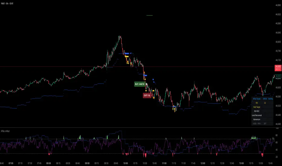
Rifle UnifiedThis script is designed for use on 30-second charts of Dow Jones-related symbols (YM, MYM, US30). It provides automated buy and sell signals using a combination of price action, RSI (Relative Strength Index), and volume analysis. The script is intended for both live trading signals and backtesting, with configurable risk management and debugging features.
Core Functionality
1. Signal Generation Logic
Trigger: The algorithm looks for a sharp price move (drop or rise) of a user-defined threshold (default: 80 points) within a specified lookback window (default: 20 minutes).
Levels: It monitors for price drops below specific numerical levels ending in 23, 43, or 73 (e.g., 42223, 42273).
RSI Condition: When price falls below one of these levels and the RSI is below 30, the setup is considered active.
Buy Signal: A buy is triggered if, after setup:
Price rises back above the level,
The RSI rate of change (ROC) indicates exhaustion of the drop,
The current bar shows positive momentum.
2. Trade Management
Stop Loss & Take Profit: Configurable fixed or trailing stop loss and take profit levels are plotted and managed automatically.
Exit Signals: The script signals exit based on price action relative to these risk management levels.
3. Filters & Enhancements
Parabolic Move Filter: Prevents entries during extreme price moves.
Dead Cat Bounce Filter: Avoids false signals after sharp reversals.
Volume Filter: Optionally requires volume conditions for trade entries (especially for shorts).
Multiple Confirmation Layers : Includes checks for 5-minute RSI, momentum, and price retracement.
User Inputs & Customization
Trade Direction: Toggle between LONG and SHORT signal generation.
Trigger Settings: Adjust thresholds for price moves, lookback windows, RSI ROC, and volume requirements.
Trade Settings: Set take profit, stop loss, and trailing stop behavior.
Debug & Visualization: Enable or disable various plots, labels, and debug tables for in-depth analysis.
Backtesting: Integrated backtester with summary and detailed statistics tables.
Technical Features
Uses External Libraries: Relies on RifleShooterLib for core logic and BackTestLib for backtesting and statistics.
Multi-timeframe Analysis: Incorporates both 30-second and 5-minute RSI calculations.
Chart Annotations: Plots entry/exit points, risk levels, and debug information directly on the chart.
Alert Conditions: Built-in alert triggers for key events (initial move, stall, entry).
Intended Use
Markets: Dow Jones symbols (YM, MYM, US30, or US30 CFD).
Timeframe: 30-second chart.
Purpose: Automated signal generation for discretionary or algorithmic trading, with robust risk management and backtesting support.
Notable Customization & Extension Points
Momentum Calculation: Plans to replace the current momentum measure with "sqz momentum".
Displacement Logic: Future update to use "FVG concept" for displacement.
High-Contrast RSI: Optional visual enhancements for RSI extremes.
Time-based Stop: Consideration for adding a time-based stop mechanism.
This script is highly modular, with extensive user controls, and is suitable for both live trading and historical analysis of Dow Jones index movements
Red Report Filter x 'Bull_Trap_9'Hello Traders!
This one is my favorite.
This is indicator / filter: '2 of 2.'
'1 of 2' is the, 'Closed Market Filter,' I posted before this that you may like.
Again, I prefer 'Filter' over 'Indicator' because this Pine Script code does not interact with the actual price data.
It makes handling high impact reports effortless.
As you all know; if you're on a Prop and breach a 'Red,' you lose your account.
This will filter up to 5 reports. More than enough unless you're on EURUSD!
It offers both 'Red' and 'Orange' report control.
The default window times of 15 / 6 are programmed for red events. You can always alter the base code for your desired, 'Before / After.'
Click the tooltip for more info.
How to use:
You do need to update the inputs daily with the current report times before each open.
I trade YM / US markets. Those reports are very repetitive on their delivery times, so I usually leave a 10:00 setting in slot 1. I then toggle it 'On' or 'Off' per demand.
Just open the dialogue box and it is pretty self explanatory.
I used task scheduler for a lot of years, but that wasn't very reliable, modest work to set up daily and a lot of times I may not hear it or it malfunctions because of a Windows update.
TradingView has the little icon that floats from the bottom right, but who really looks for that.
Any audio alert is subject to fail for a number of reasons.
This filter REDS the screen in your face. Leaves no doubt about what's coming.
I know there may be other apps and options out there, but this filter is integral to the TradingView chart itself embedded through Pine Script. It is right there, a click away, easy to input data, and as long as your chart is active and working, the filter will fire.
I did not build an alert condition into this, but I'm sure that could be an option if you want to program in audio as well.
Please Note: Only when the price candles push into the filter zone, will the filter start to display. Run a test a minute from the current price candle and you can see how it functions.
I appreciate your interest.

Intraday & Annual CAPM AlphaIntraday & Annual CAPM Alpha
This TradingView™ Pine v6 indicator computes and plots a stock’s CAPM α (alpha) on both intraday and daily/annualized timeframes, allowing you to monitor relative performance against a chosen benchmark (e.g. SPX, NDX).
⸻
Key Outputs
1. Intraday α per Bar (blue line)
• Calculates α from a rolling-window linear regression of the last N bars’ returns (default 60).
• Expressed as “extra return per bar” vs. the benchmark.
2. Intraday α Daily-Equivalent (stepped blue line)
• Scales the per-bar α to a full trading day (390 minutes), showing “if this pace held all day, outperformance (%)”.
3. Annualized α (yellow line)
• Performs the same CAPM regression on daily returns over a D-day lookback (default 252), then annualizes α by multiplying by 252.
• Indicates longer-term relative strength/weakness vs. the benchmark.
⸻
Inputs
• Benchmark Symbol: Choose any index or ETF (e.g. “SPX”, “NDX”).
• Intraday Lookback Bars: Number of bars for intraday α regression (default 60).
• Daily Lookback Days: Number of trading days for daily CAPM regression (default 252).
• Use Log Returns?: Toggle between arithmetic vs. log returns.
⸻
How to Use
• Short-Term Signals:
• Watch the blue α/bar line on 1–15 min charts. A cross from negative to positive suggests intraday outperformance; a reversal warns of weakening momentum.
• The blue daily-equivalent α gives a smoother view—e.g. > +1% signals strong intraday bias, < –1% signals underperformance.
• Long-Term Trends:
• On daily charts, focus on the yellow annualized α. A sustained positive α implies this stock has historically beaten the benchmark; sustained negative α implies the opposite.
• Combining Timeframes:
• Use intraday α for timing entries/exits within the session, and annualized α to confirm whether you want a bullish or bearish bias over days to weeks.
⸻
Install & Configure
1. Copy the Pine v6 script into the TradingView Pine Editor.
2. Set your favorite benchmark, lookback periods, and returns type.
3. Add to your chart to start visualizing real-time CAPM α signals!
Feel free to adjust the lookback windows and threshold levels to suit your trading style.

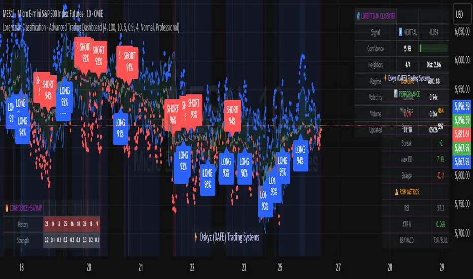
Lorentzian Classification - Advanced Trading DashboardLorentzian Classification - Relativistic Market Analysis
A Journey from Theory to Trading Reality
What began as fascination with Einstein's relativity and Lorentzian geometry has evolved into a practical trading tool that bridges theoretical physics and market dynamics. This indicator represents months of wrestling with complex mathematical concepts, debugging intricate algorithms, and transforming abstract theory into actionable trading signals.
The Theoretical Foundation
Lorentzian Distance in Market Space
Traditional Euclidean distance treats all feature differences equally, but markets don't behave uniformly. Lorentzian distance, borrowed from spacetime geometry, provides a more nuanced similarity measure:
d(x,y) = Σ ln(1 + |xi - yi|)
This logarithmic formulation naturally handles:
Scale invariance: Large price moves don't overwhelm small but significant patterns
Outlier robustness: Extreme values are dampened rather than dominating
Non-linear relationships: Captures market behavior better than linear metrics
K-Nearest Neighbors with Relativistic Weighting
The algorithm searches historical market states for patterns similar to current conditions. Each neighbor receives weight inversely proportional to its Lorentzian distance:
w = 1 / (1 + distance)
This creates a "gravitational" effect where closer patterns have stronger influence on predictions.
The Implementation Challenge
Creating meaningful market features required extensive experimentation:
Price Features: Multi-timeframe momentum (1, 2, 3, 5, 8 bar lookbacks) Volume Features: Relative volume analysis against 20-period average
Volatility Features: ATR and Bollinger Band width normalization Momentum Features: RSI deviation from neutral and MACD/price ratio
Each feature undergoes min-max normalization to ensure equal weighting in distance calculations.
The Prediction Mechanism
For each current market state:
Feature Vector Construction: 12-dimensional representation of market conditions
Historical Search: Scan lookback period for similar patterns using Lorentzian distance
Neighbor Selection: Identify K nearest historical matches
Outcome Analysis: Examine what happened N bars after each match
Weighted Prediction: Combine outcomes using distance-based weights
Confidence Calculation: Measure agreement between neighbors
Technical Hurdles Overcome
Array Management: Complex indexing to prevent look-ahead bias
Distance Calculations: Optimizing nested loops for performance
Memory Constraints: Balancing lookback depth with computational limits
Signal Filtering: Preventing clustering of identical signals
Advanced Dashboard System
Main Control Panel
The primary dashboard provides real-time market intelligence:
Signal Status: Current prediction with confidence percentage
Neighbor Analysis: How many historical patterns match current conditions
Market Regime: Trend strength, volatility, and volume analysis
Temporal Context: Real-time updates with timestamp
Performance Analytics
Comprehensive tracking system monitors:
Win Rate: Percentage of successful predictions
Signal Count: Total predictions generated
Streak Analysis: Current winning/losing sequence
Drawdown Monitoring: Maximum equity decline
Sharpe Approximation: Risk-adjusted performance estimate
Risk Assessment Panel
Multi-dimensional risk analysis:
RSI Positioning: Overbought/oversold conditions
ATR Percentage: Current volatility relative to price
Bollinger Position: Price location within volatility bands
MACD Alignment: Momentum confirmation
Confidence Heatmap
Visual representation of prediction reliability:
Historical Confidence: Last 10 periods of prediction certainty
Strength Analysis: Magnitude of prediction values over time
Pattern Recognition: Color-coded confidence levels for quick assessment
Input Parameters Deep Dive
Core Algorithm Settings
K Nearest Neighbors (1-20): More neighbors create smoother but less responsive signals. Optimal range 5-8 for most markets.
Historical Lookback (50-500): Deeper history improves pattern recognition but reduces adaptability. 100-200 bars optimal for most timeframes.
Feature Window (5-30): Longer windows capture more context but reduce sensitivity. Match to your trading timeframe.
Feature Selection
Price Changes: Essential for momentum and reversal detection Volume Profile: Critical for institutional activity recognition Volatility Measures: Key for regime change detection Momentum Indicators: Vital for trend confirmation
Signal Generation
Prediction Horizon (1-20): How far ahead to predict. Shorter horizons for scalping, longer for swing trading.
Signal Threshold (0.5-0.9): Confidence required for signal generation. Higher values reduce false signals but may miss opportunities.
Smoothing (1-10): EMA applied to raw predictions. More smoothing reduces noise but increases lag.
Visual Design Philosophy
Color Themes
Professional: Corporate blue/red for institutional environments Neon: Cyberpunk cyan/magenta for modern aesthetics
Matrix: Green/red hacker-inspired palette Classic: Traditional trading colors
Information Hierarchy
The dashboard system prioritizes information by importance:
Primary Signals: Largest, most prominent display
Confidence Metrics: Secondary but clearly visible
Supporting Data: Detailed but unobtrusive
Historical Context: Available but not distracting
Trading Applications
Signal Interpretation
Long Signals: Prediction > threshold with high confidence
Look for volume confirmation
- Check trend alignment
- Verify support levels
Short Signals: Prediction < -threshold with high confidence
Confirm with resistance levels
- Check for distribution patterns
- Verify momentum divergence
- Market Regime Adaptation
Trending Markets: Higher confidence in directional signals
Ranging Markets: Focus on reversal signals at extremes
Volatile Markets: Require higher confidence thresholds
Low Volume: Reduce position sizes, increase caution
Risk Management Integration
Confidence-Based Sizing: Larger positions for higher confidence signals
Regime-Aware Stops: Wider stops in volatile regimes
Multi-Timeframe Confirmation: Align signals across timeframes
Volume Confirmation: Require volume support for major signals
Originality and Innovation
This indicator represents genuine innovation in several areas:
Mathematical Approach
First application of Lorentzian geometry to market pattern recognition. Unlike Euclidean-based systems, this naturally handles market non-linearities.
Feature Engineering
Sophisticated multi-dimensional feature space combining price, volume, volatility, and momentum in normalized form.
Visualization System
Professional-grade dashboard system providing comprehensive market intelligence in intuitive format.
Performance Tracking
Real-time performance analytics typically found only in institutional trading systems.
Development Journey
Creating this indicator involved overcoming numerous technical challenges:
Mathematical Complexity: Translating theoretical concepts into practical code
Performance Optimization: Balancing accuracy with computational efficiency
User Interface Design: Making complex data accessible and actionable
Signal Quality: Filtering noise while maintaining responsiveness
The result is a tool that brings institutional-grade analytics to individual traders while maintaining the theoretical rigor of its mathematical foundation.
Best Practices
- Parameter Optimization
- Start with default settings and adjust based on:
Market Characteristics: Volatile vs. stable
Trading Timeframe: Scalping vs. swing trading
Risk Tolerance: Conservative vs. aggressive
Signal Confirmation
Never trade on Lorentzian signals alone:
Price Action: Confirm with support/resistance
Volume: Verify with volume analysis
Multiple Timeframes: Check higher timeframe alignment
Market Context: Consider overall market conditions
Risk Management
Position Sizing: Scale with confidence levels
Stop Losses: Adapt to market volatility
Profit Targets: Based on historical performance
Maximum Risk: Never exceed 2-3% per trade
Disclaimer
This indicator is for educational and research purposes only. It does not constitute financial advice or guarantee profitable trading results. The Lorentzian classification system reveals market patterns but cannot predict future price movements with certainty. Always use proper risk management, conduct your own analysis, and never risk more than you can afford to lose.
Market dynamics are inherently uncertain, and past performance does not guarantee future results. This tool should be used as part of a comprehensive trading strategy, not as a standalone solution.
Bringing the elegance of relativistic geometry to market analysis through sophisticated pattern recognition and intuitive visualization.
Thank you for sharing the idea. You're more than a follower, you're a leader!
@vasanthgautham1221
Trade with precision. Trade with insight.
— Dskyz , for DAFE Trading Systems
Multi-Session ORBThe Multi-Session ORB Indicator is a customizable Pine Script (version 6) tool designed for TradingView to plot Opening Range Breakout (ORB) levels across four major trading sessions: Sydney, Tokyo, London, and New York. It allows traders to define specific ORB durations and session times in Central Daylight Time (CDT), making it adaptable to various trading strategies.
Key Features:
1. Customizable ORB Duration: Users can set the ORB duration (default: 15 minutes) via the inputMax parameter, determining the time window for calculating the high and low of each session’s opening range.
2. Flexible Session Times: The indicator supports user-defined session and ORB times for:
◦ Sydney: Default ORB (17:00–17:15 CDT), Session (17:00–01:00 CDT)
◦ Tokyo: Default ORB (19:00–19:15 CDT), Session (19:00–04:00 CDT)
◦ London: Default ORB (02:00–02:15 CDT), Session (02:00–11:00 CDT)
◦ New York: Default ORB (08:30–08:45 CDT), Session (08:30–16:00 CDT)
3. Session-Specific ORB Levels: For each session, the indicator calculates and tracks the high and low prices during the specified ORB period. These levels are updated dynamically if new highs or lows occur within the ORB timeframe.
4. Visual Representation:
◦ ORB high and low lines are plotted only during their respective session times, ensuring clarity.
◦ Each session’s lines are color-coded for easy identification:
▪ Sydney: Light Yellow (high), Dark Yellow (low)
▪ Tokyo: Light Pink (high), Dark Pink (low)
▪ London: Light Blue (high), Dark Blue (low)
▪ New York: Light Purple (high), Dark Purple (low)
◦ Lines are drawn with a linewidth of 2 and disappear when the session ends or if the timeframe is not intraday (or exceeds the ORB duration).
5. Intraday Compatibility: The indicator is optimized for intraday timeframes (e.g., 1-minute to 15-minute charts) and only displays when the chart’s timeframe multiplier is less than or equal to the ORB duration.
How It Works:
• Session Detection: The script uses the time() function to check if the current bar falls within the user-defined ORB or session time windows, accounting for all days of the week.
• ORB Logic: At the start of each session’s ORB period, the script initializes the high and low based on the first bar’s prices. It then updates these levels if subsequent bars within the ORB period exceed the current high or fall below the current low.
• Plotting: ORB levels are plotted as horizontal lines during the respective session, with visibility controlled to avoid clutter outside session times or on incompatible timeframes.
Use Case:
Traders can use this indicator to identify key breakout levels for each trading session, facilitating strategies based on price action around the opening range. The flexibility to adjust ORB and session times makes it suitable for various markets (e.g., forex, stocks, or futures) and time zones.
Limitations:
• The indicator is designed for intraday timeframes and may not display on higher timeframes (e.g., daily or weekly) or if the timeframe multiplier exceeds the ORB duration.
• Time inputs are in CDT, requiring users to adjust for their local timezone or market requirements.
• If you need to use this for GC/CL/SPY/QQQ you have to adjust the times by one hour.
This indicator is ideal for traders focusing on session-based breakout strategies, offering clear visualization and customization for global market sessions.

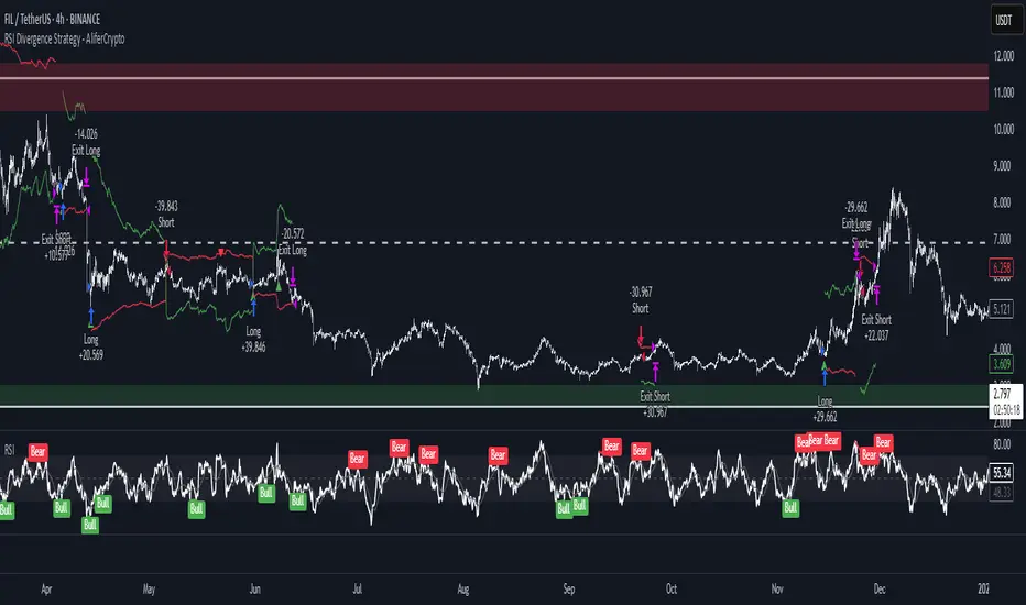
RSI Divergence Strategy - AliferCryptoStrategy Overview
The RSI Divergence Strategy is designed to identify potential reversals by detecting regular bullish and bearish divergences between price action and the Relative Strength Index (RSI). It automatically enters positions when a divergence is confirmed and manages risk with configurable stop-loss and take-profit levels.
Key Features
Automatic Divergence Detection: Scans for RSI pivot lows/highs vs. price pivots using user-defined lookback windows and bar ranges.
Dual SL/TP Methods:
- Swing-based: Stops placed a configurable percentage beyond the most recent swing high/low.
- ATR-based: Stops placed at a multiple of Average True Range, with a separate risk/reward multiplier.
Long and Short Entries: Buys on bullish divergences; sells short on bearish divergences.
Fully Customizable: Input groups for RSI, divergence, swing, ATR, and general SL/TP settings.
Visual Plotting: Marks divergences on chart and plots stop-loss (red) and take-profit (green) lines for active trades.
Alerts: Built-in alert conditions for both bullish and bearish RSI divergences.
Detailed Logic
RSI Calculation: Computes RSI of chosen source over a specified period.
Pivot Detection:
- Identifies RSI pivot lows/highs by scanning a lookback window to the left and right.
- Uses ta.barssince to ensure pivots are separated by a minimum/maximum number of bars.
Divergence Confirmation:
- Bullish: Price makes a lower low while RSI makes a higher low.
- Bearish: Price makes a higher high while RSI makes a lower high.
Entry:
- Opens a Long position when bullish divergence is true.
- Opens a Short position when bearish divergence is true.
Stop-Loss & Take-Profit:
- Swing Method: Computes the recent swing high/low then adjusts by a percentage margin.
- ATR Method: Uses the current ATR × multiplier applied to the entry price.
- Take-Profit: Calculated as entry price ± (risk × R/R ratio).
Exit Orders: Uses strategy.exit to place bracket orders (stop + limit) for both long and short positions.
Inputs and Configuration
RSI Settings: Length & price source for the RSI.
Divergence Settings: Pivot lookback parameters and valid bar ranges.
SL/TP Settings: Choice between Swing or ATR method.
Swing Settings: Swing lookback length, margin (%), and risk/reward ratio.
ATR Settings: ATR length, stop multiplier, and risk/reward ratio.
Usage Notes
Adjust the Pivot Lookback and Range values to suit the volatility and timeframe of your market.
Use higher ATR multipliers for wider stops in choppy conditions, or tighten swing margins in trending markets.
Backtest different R/R ratios to find the balance between win rate and reward.
Disclaimer
This script is for educational purposes only and does not constitute financial advice. Trading carries significant risk and you may lose more than your initial investment. Always conduct your own research and consider consulting a professional before making any trading decisions.
ICT SMC Liquidity Grabs and OBsICT SMC Liquidity Grabs + Order Blocks + Fibonacci OTE Levels
A High-Probability Entry Engine for Smart Money Concept Traders
This script combines three powerful Smart Money Concepts (SMC) into a single tool: Liquidity Grabs, Order Block Zones, and Fibonacci OTE Levels, allowing traders to identify institutional entry models with clean, rule-based visual signals.
It’s designed to simplify SMC trading by highlighting confluence zones where price is likely to reverse or continue — with clear visual zones, entry arrows, and take profit projections.
🔍 What This Script Does:
Detects Liquidity Grabs
Identifies when price sweeps above/below the highest high or lowest low within a user-defined lookback period and closes back inside.
Plots orange labels on the chart to signal potential liquidity events (LG-H / LG-L).
Plots Order Blocks After Liquidity Grabs
After a liquidity grab, the script looks for displacement candles (strong bullish or bearish moves) and draws highlighted OB zones extending several bars to the right.
These zones represent potential institutional footprints for price reversals.
Draws Fibonacci OTE Levels (Optimal Trade Entry)
Uses recent swing high and low pivots to automatically calculate OTE zones (default: 62% and 75% retracement levels).
Draws these retracement zones for both bullish and bearish setups.
Marks Valid OTE Entry Zones
Buy/Sell zones only trigger when:
A liquidity grab occurs,
Price enters the OTE zone,
And a strong confirming candle is present.
Plots green/red arrows for valid buy/sell OTE entries.
Auto-Draws Take Profit Zones
TP1 = Previous swing high/low
TP2 = Risk-based R-multiplied extension (e.g., 1.5R — customizable)
Alerts
Triggers alerts when valid buy or sell OTE setups are detected.
⚙️ Customization Features:
Toggle each feature: Liquidity Grabs, Order Blocks, Fibonacci OTE levels
Set Fibonacci retracement percentages (e.g., 0.62 / 0.75)
Adjust lookback window for liquidity detection
Customize the take-profit multiplier (R-based)
Full control over visuals: colors, labels, and lines
💡 How to Use:
Use this script to scan for high-confluence trade setups based on Smart Money principles.
Combine with session timing (e.g., New York open), major swing structure, or Kill Zone windows for maximum edge.
Look for arrows inside OB zones or OTE levels following liquidity sweeps for cleaner entries.
🔗 Works Best With:
✅ First FVG — Opening Range Fair Value Gap Detector: Identify early inefficiencies to set the narrative for the day.
✅ Liquidity Levels — Smart Swing Lows: Spot key structural lows that can fuel stop hunts and reversals.
✅ ICT Turtle Soup — Liquidity Reversal: Add a classic reversal pattern to your toolkit to catch fakeouts cleanly.
Together, these tools build a complete Smart Money ecosystem for entry precision, risk management, and price behavior forecasting.

ICT MACRO MAX RETRI ( ALERT )🖤 ICT Reversal Detector – Minimalist Edition
This indicator is designed for traders who follow Inner Circle Trader (ICT) concepts, particularly focused on liquidity sweeps and displacement reversals.
It detects:
• Swing Highs & Lows that occur during the most reactive windows of each hour
→ Specifically the last 20 minutes and first 15 minutes
(ICT teaches these moments often reveal macro-level reversals. I’ve expanded the window slightly to give the indicator more room to catch valid setups.)
• Liquidity Sweeps of previous highs/lows
• Displacement (State Change): defined as a manipulation wick followed by 1–3 strong candles closing in the opposite direction
Visually:
• Clean black lines pointing right from the liquidity sweep wick
• White triangle markers inside black label boxes only when valid displacement occurs
• No clutter, no unnecessary shapes — just focused signal
Built for:
• 5-minute charts, especially NASDAQ (NAS100) and S&P 500 (SPX500)
• Confirm setups manually on the 15-minute chart for extra precision
This is a partial automation tool for ICT-style reversal traders who prefer clarity, minimalism, and sharp intuition over noise.
Let it alert you to setups — then decide like a sniper.

Reversal Signals [AlgoAlpha]📈🔄 Reversal Signals – Master Market Reversals with Precision! 🚀✨
Elevate your trading strategy with the Reversal Signals indicator by AlgoAlpha. This advanced tool is designed to pinpoint potential bullish and bearish reversals by analyzing price action and, optionally, volume confirmations. It seamlessly combines reversal detection with trend analysis, giving you a comprehensive view of market dynamics to make informed trading decisions.
Key Features
🔎 Price Action Reversal Detection : Identifies potential reversal points by comparing current price movements against historical candle patterns within a customizable lookback period.
📊 Volume Confirmation : Optionally integrates volume analysis to confirm the strength of reversal signals, enhancing their reliability.
📈 Stepped Moving Average Trend Indicator : Employs a stepped moving average that adjusts at set intervals to reflect underlying market trends.
⚙️ Customizable Settings : Tailor the indicator to your trading style with adjustable parameters for lookback periods, confirmation windows, moving average types, and more.
🎨 Visual Signals and Trend Coloring : Clear on-chart labels for reversal signals and color-coded trend areas to quickly identify bullish and bearish conditions.
🔔 Alerts for Key Market Events : Set up custom alerts for reversal signals and trend shifts to stay ahead of market movements.
Quick Guide to Using the Reversal Signals Indicator :
🛠 Add the Indicator : Add the indicator to your favorites by pressing the star icon. Customize settings like Candle Lookback, Confirm Within, and Use Volume Confirmation to fit your trading style.
📊 Market Analysis : Observe the "𝓡" labels on the chart indicating bullish and bearish reversal signals. Look for labels below the bars for bullish signals and above the bars for bearish signals. Use the color-filled areas between the stepped moving average and the center line to assess market trends.
🔔 Alerts : Enable notifications for reversal signals and trend shifts to stay informed about market movements without constantly monitoring the chart.
How It Works
The Reversal Signals indicator operates by conducting a thorough analysis of price action over a user-defined lookback period. For a bullish reversal, the indicator checks if the current closing price is lower than the lows of the preceding candles within the lookback window, suggesting a potential oversold condition. If this criterion is met, it marks the candle as a potential reversal point and waits for confirmation within a specified number of subsequent candles. Confirmation occurs when the price rises above the high of the identified candle, signaling a bullish reversal. An optional volume confirmation can be enabled to ensure that the reversal is supported by higher-than-average trading volume, adding an extra layer of validation to the signal. The process is mirrored for bearish reversals, where the indicator looks for the closing price exceeding previous highs and awaits confirmation of a downward move.
Complementing the reversal signals, the indicator features a stepped moving average that serves as a dynamic trend indicator. This moving average updates at intervals defined by the MA Step Period and shifts direction based on price crossings. If the price remains above the stepped MA, it indicates a bullish trend, coloring the area between the MA and the center line in green. Conversely, if the price falls below the stepped MA, a bearish trend is signaled, and the area is shaded red. This visual representation helps traders quickly assess the prevailing market trend and align their trading decisions accordingly.
Experience a new level of market insight with the Reversal Signals indicator. Add it to your TradingView chart today and enhance your ability to detect and act on key ma

Enhanced Market Analyzer with Adaptive Cognitive LearningThe "Enhanced Market Analyzer with Advanced Features and Adaptive Cognitive Learning" is an advanced, multi-dimensional trading indicator that leverages sophisticated algorithms to analyze market trends and generate predictive trading signals. This indicator is designed to merge traditional technical analysis with modern machine learning techniques, incorporating features such as adaptive learning, Monte Carlo simulations, and probabilistic modeling. It is ideal for traders who seek deeper market insights, adaptive strategies, and reliable buy/sell signals.
Key Features:
Adaptive Cognitive Learning:
Utilizes Monte Carlo simulations, reinforcement learning, and memory feedback to adapt to changing market conditions.
Adjusts the weighting and learning rate of signals dynamically to optimize predictions based on historical and real-time data.
Hybrid Technical Indicators:
Custom RSI Calculation: An RSI that adapts its length based on recursive learning and error adjustments, making it responsive to varying market conditions.
VIDYA with CMO Smoothing: An advanced moving average that incorporates Chander Momentum Oscillator for adaptive smoothing.
Hamming Windowed VWMA: A volume-weighted moving average that applies a Hamming window for smoother calculations.
FRAMA: A fractal adaptive moving average that responds dynamically to price movements.
Advanced Statistical Analysis:
Skewness and Kurtosis: Provides insights into the distribution and potential risk of market trends.
Z-Score Calculations: Identifies extreme market conditions and adjusts trading thresholds dynamically.
Probabilistic Monte Carlo Simulation:
Runs thousands of simulations to assess potential price movements based on momentum, volatility, and volume factors.
Integrates the results into a probabilistic signal that informs trading decisions.
Feature Extraction:
Calculates a variety of market metrics, including price change, momentum, volatility, volume change, and ATR.
Normalizes and adapts these features for use in machine learning algorithms, enhancing signal accuracy.
Ensemble Learning:
Combines signals from different technical indicators, such as RSI, MACD, Bollinger Bands, Stochastic Oscillator, and statistical features.
Weights each signal based on cumulative performance and learning feedback to create a robust ensemble signal.
Recursive Memory and Feedback:
Stores and averages past RSI calculations in a memory array to provide historical context and improve future predictions.
Adaptive memory factor adjusts the influence of past data based on current market conditions.
Multi-Factor Dynamic Length Calculation:
Determines the length of moving averages based on volume, volatility, momentum, and rate of change (ROC).
Adapts to various market conditions, ensuring that the indicator is responsive to both high and low volatility environments.
Adaptive Learning Rate:
The learning rate can be adjusted based on market volatility, allowing the system to adapt its speed of learning and sensitivity to changes.
Enhances the system's ability to react to different market regimes.
Monte Carlo Simulation Engine:
Simulates thousands of random outcomes to model potential future price movements.
Weights and aggregates these simulations to produce a final probabilistic signal, providing a comprehensive risk assessment.
RSI with Dynamic Adjustments:
The initial RSI length is adjusted recursively based on calculated errors between true RSI and predicted RSI.
The adaptive RSI calculation ensures that the indicator remains effective across various market phases.
Hybrid Moving Averages:
Short-Term and Long-Term Averages: Combines FRAMA, VIDYA, and Hamming VWMA with specific weights for a unique hybrid moving average.
Weighted Gradient: Applies a color gradient to indicate trend strength and direction, improving visual clarity.
Signal Generation:
Generates buy and sell signals based on the ensemble model and multi-factor analysis.
Uses percentile-based thresholds to determine overbought and oversold conditions, factoring in historical data for context.
Optional settings to enable adaptation to volume and volatility, ensuring the indicator remains effective under different market conditions.
Monte Carlo and Learning Parameters:
Users can customize the number of Monte Carlo simulations, learning rate, memory factor, and reward decay for tailored performance.
Applications:
Scalping and Day Trading:
The fast response of the adaptive RSI and ensemble learning model makes this indicator suitable for short-term trading strategies.
Swing Trading:
The combination of long-term moving averages and probabilistic models provides reliable signals for medium-term trends.
Volatility Analysis:
The ATR, Bollinger Bands, and adaptive moving averages offer insights into market volatility, helping traders adjust their strategies accordingly.
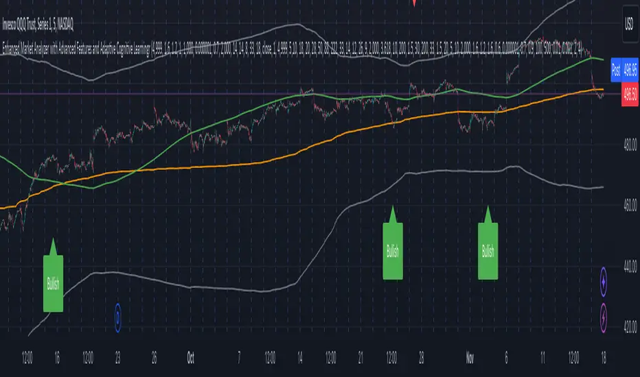
Standard Deviation OscillatorStandard Deviation Oscillator (STDEV OSC) v1.1
Description
The Standard Deviation Oscillator transforms traditional volatility measurements into a dynamic oscillator that fluctuates between 0 and 100. This advanced technical analysis tool helps traders identify periods of extreme volatility and potential market turning points.
Features
Normalized volatility readings (0-100 scale)
Dynamic color changes based on volatility levels
Customizable overbought/oversold thresholds
Built-in alert conditions
Adaptive calculation using rolling windows
Clean, professional visualization
Indicator Parameters
Length: 20; Calculation period for standard deviation
Source: close; Price source for calculations
Overbought Level: 70; Upper threshold for high volatility
Oversold Level: 30; Lower threshold for low volatility
Visual Components
- Main Oscillator Line: Changes color based on current level
- Red: Above overbought level
- Green: Below oversold level
- Blue: Normal range
- Reference Lines:
- Overbought level (default: 70)
- Oversold level (default: 30)
- Middle line (50)
Alert Conditions
1. Volatility High Alert
- Triggers when oscillator crosses above the overbought level
- Useful for identifying potential market tops or breakout scenarios
2. Volatility Low Alert
- Triggers when oscillator crosses below the oversold level
- Helps identify potential market bottoms or consolidation periods
Risk Adjustment Tool
- Scale position sizes inversely to oscillator readings
- Reduce exposure during extremely high volatility periods
- Increase position sizes during normal volatility conditions
Best Practices
1. Timeframe Selection
- Best suited for 1H, 4H, and Daily charts
- Adjust length parameter based on timeframe
2. Confirmation
- Use in conjunction with trend indicators
- Confirm signals with price action patterns
- Consider overall market context
3. Parameter Optimization
- Backtest different length settings
- Adjust overbought/oversold levels based on asset
- Consider market conditions when setting alerts
Technical Notes
- Built in PineScript v5
- Optimized for TradingView platform
- Uses rolling window calculations for better adaptability
- Compatible with all trading instruments
- Minimal performance impact on charts
Version History
- v1.1: Added dynamic coloring, customizable levels, and alert conditions
- v1.0: Initial release with basic oscillator functionality
Disclaimer
This technical indicator is provided for educational and informational purposes only. Past performance is not indicative of future results. Always conduct thorough testing and use proper risk management techniques.
---
Tags: #TechnicalAnalysis #Volatility #Trading #Oscillator #TradingView #PineScript

ICT Silver Bullet with signals
The "ICT Silver Bullet with signals" indicator (inspired from the lectures of "The Inner Circle Trader" (ICT)),
goes a step further than the ICT Silver Bullet publication, which I made for LuxAlgo :
• uses HTF candles
• instant drawing of Support & Resistance (S/R) lines when price retraces into FVG
• NWOG - NDOG S/R lines
• signals
The Silver Bullet (SB) window which is a specific 1-hour interval where a Fair Value Gap (FVG) pattern can be formed.
When price goes back to the FVG, without breaking it, Support & Resistance lines will be drawn immediately.
There are 3 different Silver Bullet windows (New York local time):
The London Open Silver Bullet (03 AM — 04 AM ~ 03:00 — 04:00)
The AM Session Silver Bullet (10 AM — 11 AM ~ 10:00 — 11:00)
The PM Session Silver Bullet (02 PM — 03 PM ~ 14:00 — 15:00)
🔶 USAGE
This technique can visualise potential support/resistance lines, which can be used as targets.
The script contains 2 main components:
• forming of a Fair Value Gap (FVG)
• drawing support/resistance (S/R) lines
🔹 Forming of FVG
When HTF candles forms an FVG, the FVG will be drawn at the end (close) of the last HTF candle.
To make it easier to visualise the 2 HTF candles that form the FVG, you can enable
• SHOW -> HTF candles
During the SB session, when a FVG is broken, the FVG will be removed, together with its S/R lines.
The same goes if price did not retrace into FVG at the last bar of the SB session
Only exception is when "Remove broken FVG's" is disabled.
In this case a FVG can be broken, as long as price bounces back before the end of the SB session, it will remain to be visible:
🔹 Drawing support/resistance lines
S/R target lines are drawn immediately when price retraces into the FVG.
They will remain updated until they are broken (target hit)
Potential S/R lines are formed by:
• previous swings (swing settings (left-right)
• New Week Opening Gap (NWOG): close on Friday - weekly open
• New Day Opening Gap (NWOG): close previous day - current daily open
Only non-broken lines are included.
Broken =
• minimum of open and close below potential S/R line
• maximum of open and close above potential S/R line
NDOG lines are coloured fuchsia (as in the ICT lectures), NWOG are coloured white (darkmode) or black (lightmode ~ ICT lectures)
Swing line colour can be set as desired.
Here S/R includes NDOG lines:
The same situation, with "Extend Target-lines to their source" enabled:
Here with NWOG lines:
This publication contains a "Minimum Trade Framework (mTFW)", which represents the best-case expected price delivery, this is not your actual trade entry - exit range.
• 40 ticks for index futures or indices
• 15 pips for Forex pairs
The minimum distance (if applicable) can be shown by enabling "Show" - "Minimum Trade Framework" -> blue arrow from close to mTFW
Potential S/R lines needs to be higher (bullish) or lower (bearish) than mTFW.
🔶 SETTINGS
(check USAGE for deeper insights and explanation)
🔹 Only last x bars: when enabled, the script will do most of the calculations at these last x candles, potentially this can speeds calculations.
🔹 Swing settings (left-right): Sets the length, which will set the lookback period/sensitivity of the ZigZag patterns (which directs the trend and points for S/R lines)
🔹 FVG
HTF (minutes): 1-15 minutes.
• When the chart TF is equal of higher, calculations are based on current TF.
• Chart TF > 15 minutes will give the warning: "Please use a timeframe <= 15 minutes".
Remove broken FVG's: when enabled the script will remove FVG (+ associated S/R lines) immediately when FVG is broken at opposite direction.
FVG's still will be automatically removed at the end of the SB session, when there is no retrace, together with associated S/R lines,...
~ trend: Only include FVG in the same direction as the current trend
Note -> when set 'right' (swing setting) rather high ( > 3), he trend change will be delayed as well (default 'right' max 5)
Extend: extend FVG to max right side of SB session
🔹 Targets – support/resistance
Extend Target-lines to their source: extend lines to their origin
Colours (Swing S/R lines)
🔹 Show
SB session: show lines and labels of SB session (+ colour)
• Labels can be disabled separately in the 'Style' section, colour is set at the 'Inputs' section
Trend : Show trend (ZigZag, coloured ~ trend)
HTF candles: Show the 2 HTF candles that form the FVG
Minimum Trade Framework: blue arrow (if applicable)
🔶 ALERTS
There are 4 signals provided (bullish/bearish):
FVG Formed
FVG Retrace
Target reached
FVG cancelled
You can choose between dynamic alerts - only 1 alert needs to be set for all signals, or you can set specific alerts as desired.
💜 PURPLE BARS 😈
• Since TradingView has chosen to give away our precious Purple coloured Wizard Badge, bars are coloured purple 😊😉
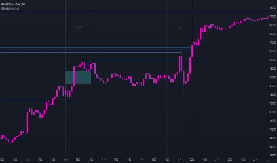
[blackcat] L2 John Ehlers Undersampled Double MALevel2
Background
This is a novel "undersampling data" processing trick proposed by John F. Ehlers in his April 2023 article "Just Ignore Them".
Function
In signal processing, undersampling, or bandpass sampling, is a technique whereby a bandpass-filtered signal is sampled at a sample rate below its Nyquist rate (twice the upper cut-off frequency), but the signal can still be reconstructed. When undersampling a bandpass signal, the samples are indistinguishable from samples of a low-frequency alias of the high-frequency signal.
John Ehlers notes that data smoothing is often used to avoid trading spikes. While this can result in fewer trading signals, it can also result in a delay in those trading signals. He describes how undersampling can be used in conjunction with Hann window finite impulse response (FIR) filters to remove high-frequency components in price data, resulting in less delay than traditional smoothing filters.
In this indicator, Hann windowing is applied a a pair of fast/slow moving averages which is used to improve their response perfomrnace. Yellow line is the fast line while fuchsia line is the slow line. You can judge bull bear stattus by checking the status it is in golden cross or in dead cross status.
Remarks
Feedbacks are appreciated.
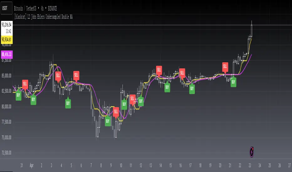
Ehlers Two-Pole Predictor [Loxx]Ehlers Two-Pole Predictor is a new indicator by John Ehlers . The translation of this indicator into PineScript™ is a collaborative effort between @cheatcountry and I.
The following is an excerpt from "PREDICTION" , by John Ehlers
Niels Bohr said “Prediction is very difficult, especially if it’s about the future.”. Actually, prediction is pretty easy in the context of technical analysis . All you have to do is to assume the market will behave in the immediate future just as it has behaved in the immediate past. In this article we will explore several different techniques that put the philosophy into practice.
LINEAR EXTRAPOLATION
Linear extrapolation takes the philosophical approach quite literally. Linear extrapolation simply takes the difference of the last two bars and adds that difference to the value of the last bar to form the prediction for the next bar. The prediction is extended further into the future by taking the last predicted value as real data and repeating the process of adding the most recent difference to it. The process can be repeated over and over to extend the prediction even further.
Linear extrapolation is an FIR filter, meaning it depends only on the data input rather than on a previously computed value. Since the output of an FIR filter depends only on delayed input data, the resulting lag is somewhat like the delay of water coming out the end of a hose after it supplied at the input. Linear extrapolation has a negative group delay at the longer cycle periods of the spectrum, which means water comes out the end of the hose before it is applied at the input. Of course the analogy breaks down, but it is fun to think of it that way. As shown in Figure 1, the actual group delay varies across the spectrum. For frequency components less than .167 (i.e. a period of 6 bars) the group delay is negative, meaning the filter is predictive. However, the filter has a positive group delay for cycle components whose periods are shorter than 6 bars.
Figure 1
Here’s the practical ramification of the group delay: Suppose we are projecting the prediction 5 bars into the future. This is fine as long as the market is continued to trend up in the same direction. But, when we get a reversal, the prediction continues upward for 5 bars after the reversal. That is, the prediction fails just when you need it the most. An interesting phenomenon is that, regardless of how far the extrapolation extends into the future, the prediction will always cross the signal at the same spot along the time axis. The result is that the prediction will have an overshoot. The amplitude of the overshoot is a function of how far the extrapolation has been carried into the future.
But the overshoot gives us an opportunity to make a useful prediction at the cyclic turning point of band limited signals (i.e. oscillators having a zero mean). If we reduce the overshoot by reducing the gain of the prediction, we then also move the crossing of the prediction and the original signal into the future. Since the group delay varies across the spectrum, the effect will be less effective for the shorter cycles in the data. Nonetheless, the technique is effective for both discretionary trading and automated trading in the majority of cases.
EXPLORING THE CODE
Before we predict, we need to create a band limited indicator from which to make the prediction. I have selected a “roofing filter” consisting of a High Pass Filter followed by a Low Pass Filter. The tunable parameter of the High Pass Filter is HPPeriod. Think of it as a “stone wall filter” where cycle period components longer than HPPeriod are completely rejected and cycle period components shorter than HPPeriod are passed without attenuation. If HPPeriod is set to be a large number (e.g. 250) the indicator will tend to look more like a trending indicator. If HPPeriod is set to be a smaller number (e.g. 20) the indicator will look more like a cycling indicator. The Low Pass Filter is a Hann Windowed FIR filter whose tunable parameter is LPPeriod. Think of it as a “stone wall filter” where cycle period components shorter than LPPeriod are completely rejected and cycle period components longer than LPPeriod are passed without attenuation. The purpose of the Low Pass filter is to smooth the signal. Thus, the combination of these two filters forms a “roofing filter”, named Filt, that passes spectrum components between LPPeriod and HPPeriod.
Since working into the future is not allowed in EasyLanguage variables, we need to convert the Filt variable to the data array XX. The data array is first filled with real data out to “Length”. I selected Length = 10 simply to have a convenient starting point for the prediction. The next block of code is the prediction into the future. It is easiest to understand if we consider the case where count = 0. Then, in English, the next value of the data array is equal to the current value of the data array plus the difference between the current value and the previous value. That makes the prediction one bar into the future. The process is repeated for each value of count until predictions up to 10 bars in the future are contained in the data array. Next, the selected prediction is converted from the data array to the variable “Prediction”. Filt is plotted in Red and Prediction is plotted in yellow.
The Predict Extrapolation indicator is shown below for the Emini S&P Futures contract using the default input parameters. Filt is plotted in red and Predict is plotted in yellow. The crossings of the Predict and Filt lines provide reliable buy and sell timing signals. There is some overshoot for the shorter cycle periods, for example in February and March 2021, but the only effect is a late timing signal. Further reducing the gain and/or reducing the BarsFwd inputs would provide better timing signals during this period.
Figure 2. Predict Extrapolation Provides Reliable Timing Signals
I have experimented with other FIR filters for predictions, but found none that had a significant advantage over linear extrapolation.
MESA
MESA is an acronym for Maximum Entropy Spectral Analysis. Conceptually, it removes spectral components until the residual is left with maximum entropy. It does this by forming an all-pole filter whose order is determined by the selected number of coefficients. It maximally addresses the data within the selected window and ignores all other data. Its resolution is determined only by the number of filter coefficients selected. Since the resulting filter is an IIR filter, a prediction can be formed simply by convolving the filter coefficients with the data. MESA is one of the few, if not the only way to practically determine the coefficients of a higher order IIR filter. Discussion of MESA is beyond the scope of this article.
TWO POLE IIR FILTER
While the coefficients of a higher order IIR filter are difficult to compute without MESA, it is a relatively simple matter to compute the coefficients of a two pole IIR filter.
(Skip this paragraph if you don’t care about DSP) We can locate the conjugate pole positions parametrically in the Z plane in polar coordinates. Let the radius be QQ and the principal angle be 360 / P2Period. The first order component is 2*QQ*Cosine(360 / P2Period) and the second order component is just QQ2. Therefore, the transfer response becomes:
H(z) = 1 / (1 - 2*QQ*Cosine(360 / P2Period)*Z-1 + QQ2*Z-2)
By mixing notation we can easily convert the transfer response to code.
Output / Input = 1 / (1 - 2*QQ*Cosine(360 / P2Period)* + QQ2* )
Output - 2*QQ*Cosine(360 / P2Period)*Output + QQ2*Output = Input
Output = Input + 2*QQ*Cosine(360 / P2Period)*Output - QQ2*Output
The Two Pole Predictor starts by computing the same “roofing filter” design as described for the Linear Extrapolation Predictor. The HPPeriod and LPPeriod inputs adjust the roofing filter to obtain the desired appearance of an indicator. Since EasyLanguage variables cannot be extended into the future, the prediction process starts by loading the XX data array with indicator data up to the value of Length. I selected Length = 10 simply to have a convenient place from which to start the prediction. The coefficients are computed parametrically from the conjugate pole positions and are normalized to their sum so the IIR filter will have unity gain at zero frequency.
The prediction is formed by convolving the IIR filter coefficients with the historical data. It is easiest to see for the case where count = 0. This is the initial prediction. In this case the new value of the XX array is formed by successively summing the product of each filter coefficient with its respective historical data sample. This process is significantly different from linear extrapolation because second order curvature is introduced into the prediction rather than being strictly linear. Further, the prediction is adaptive to market conditions because the degree of curvature depends on recent historical data. The prediction in the data array is converted to a variable by selecting the BarsFwd value. The prediction is then plotted in yellow, and is compared to the indicator plotted in red.
The Predict 2 Pole indicator is shown above being applied to the Emini S&P Futures contract for most of 2021. The default parameters for the roofing filter and predictor were used. By comparison to the Linear Extrapolation prediction of Figure 2, the Predict 2 Pole indicator has a more consistent prediction. For example, there is little or no overshoot in February or March while still giving good predictions in April and May.
Input parameters can be varied to adjust the appearance of the prediction. You will find that the indicator is relatively insensitive to the BarsFwd input. The P2Period parameter primarily controls the gain of the prediction and the QQ parameter primarily controls the amount of prediction lead during trending sections of the indicator.
TAKEAWAYS
1. A more or less universal band limited “roofing filter” indicator was used to demonstrate the predictors. The HPPeriod input parameter is used to control whether the indicator looks more like a trend indicator or more like a cycle indicator. The LPPeriod input parameter is used to control the smoothness of the indicator.
2. A linear extrapolation predictor is formed by adding the difference of the two most recent data bars to the value of the last data bar. The result is considered to be a real data point and the process is repeated to extend the prediction into the future. This is an FIR filter having a one bar negative group delay at zero frequency, but the group delay is not constant across the spectrum. This variable group delay causes the linear extrapolation prediction to be inconsistent across a range of market conditions.
3. The degree of prediction by linear extrapolation can be controlled by varying the gain of the prediction to reduce the overshoot to be about the same amplitude as the peak swing of the indicator.
4. I was unable to experimentally derive a higher order FIR filter predictor that had advantages over the simple linear extrapolation predictor.
5. A Two Pole IIR predictor can be created by parametrically locating the conjugate pole positions.
6. The Two Pole predictor is a second order filter, which allows curvature into the prediction, thus mitigating overshoot. Further, the curvature is adaptive because the prediction depends on previously computed prediction values.
7. The Two Pole predictor is more consistent over a range of market conditions.
ADDITIONS
Loxx's Expanded source types:
Library for expanded source types:
Explanation for expanded source types:
Three different signal types: 1) Prediction/Filter crosses; 2) Prediction middle crosses; and, 3) Filter middle crosses.
Bar coloring to color trend.
Signals, both Long and Short.
Alerts, both Long and Short.

Normalized, Variety, Fast Fourier Transform Explorer [Loxx]Normalized, Variety, Fast Fourier Transform Explorer demonstrates Real, Cosine, and Sine Fast Fourier Transform algorithms. This indicator can be used as a rule of thumb but shouldn't be used in trading.
What is the Discrete Fourier Transform?
In mathematics, the discrete Fourier transform (DFT) converts a finite sequence of equally-spaced samples of a function into a same-length sequence of equally-spaced samples of the discrete-time Fourier transform (DTFT), which is a complex-valued function of frequency. The interval at which the DTFT is sampled is the reciprocal of the duration of the input sequence. An inverse DFT is a Fourier series, using the DTFT samples as coefficients of complex sinusoids at the corresponding DTFT frequencies. It has the same sample-values as the original input sequence. The DFT is therefore said to be a frequency domain representation of the original input sequence. If the original sequence spans all the non-zero values of a function, its DTFT is continuous (and periodic), and the DFT provides discrete samples of one cycle. If the original sequence is one cycle of a periodic function, the DFT provides all the non-zero values of one DTFT cycle.
What is the Complex Fast Fourier Transform?
The complex Fast Fourier Transform algorithm transforms N real or complex numbers into another N complex numbers. The complex FFT transforms a real or complex signal x in the time domain into a complex two-sided spectrum X in the frequency domain. You must remember that zero frequency corresponds to n = 0, positive frequencies 0 < f < f_c correspond to values 1 ≤ n ≤ N/2 −1, while negative frequencies −fc < f < 0 correspond to N/2 +1 ≤ n ≤ N −1. The value n = N/2 corresponds to both f = f_c and f = −f_c. f_c is the critical or Nyquist frequency with f_c = 1/(2*T) or half the sampling frequency. The first harmonic X corresponds to the frequency 1/(N*T).
The complex FFT requires the list of values (resolution, or N) to be a power 2. If the input size if not a power of 2, then the input data will be padded with zeros to fit the size of the closest power of 2 upward.
What is Real-Fast Fourier Transform?
Has conditions similar to the complex Fast Fourier Transform value, except that the input data must be purely real. If the time series data has the basic type complex64, only the real parts of the complex numbers are used for the calculation. The imaginary parts are silently discarded.
What is the Real-Fast Fourier Transform?
In many applications, the input data for the DFT are purely real, in which case the outputs satisfy the symmetry
X(N-k)=X(k)
and efficient FFT algorithms have been designed for this situation (see e.g. Sorensen, 1987). One approach consists of taking an ordinary algorithm (e.g. Cooley–Tukey) and removing the redundant parts of the computation, saving roughly a factor of two in time and memory. Alternatively, it is possible to express an even-length real-input DFT as a complex DFT of half the length (whose real and imaginary parts are the even/odd elements of the original real data), followed by O(N) post-processing operations.
It was once believed that real-input DFTs could be more efficiently computed by means of the discrete Hartley transform (DHT), but it was subsequently argued that a specialized real-input DFT algorithm (FFT) can typically be found that requires fewer operations than the corresponding DHT algorithm (FHT) for the same number of inputs. Bruun's algorithm (above) is another method that was initially proposed to take advantage of real inputs, but it has not proved popular.
There are further FFT specializations for the cases of real data that have even/odd symmetry, in which case one can gain another factor of roughly two in time and memory and the DFT becomes the discrete cosine/sine transform(s) (DCT/DST). Instead of directly modifying an FFT algorithm for these cases, DCTs/DSTs can also be computed via FFTs of real data combined with O(N) pre- and post-processing.
What is the Discrete Cosine Transform?
A discrete cosine transform ( DCT ) expresses a finite sequence of data points in terms of a sum of cosine functions oscillating at different frequencies. The DCT , first proposed by Nasir Ahmed in 1972, is a widely used transformation technique in signal processing and data compression. It is used in most digital media, including digital images (such as JPEG and HEIF, where small high-frequency components can be discarded), digital video (such as MPEG and H.26x), digital audio (such as Dolby Digital, MP3 and AAC ), digital television (such as SDTV, HDTV and VOD ), digital radio (such as AAC+ and DAB+), and speech coding (such as AAC-LD, Siren and Opus). DCTs are also important to numerous other applications in science and engineering, such as digital signal processing, telecommunication devices, reducing network bandwidth usage, and spectral methods for the numerical solution of partial differential equations.
The use of cosine rather than sine functions is critical for compression, since it turns out (as described below) that fewer cosine functions are needed to approximate a typical signal, whereas for differential equations the cosines express a particular choice of boundary conditions. In particular, a DCT is a Fourier-related transform similar to the discrete Fourier transform (DFT), but using only real numbers. The DCTs are generally related to Fourier Series coefficients of a periodically and symmetrically extended sequence whereas DFTs are related to Fourier Series coefficients of only periodically extended sequences. DCTs are equivalent to DFTs of roughly twice the length, operating on real data with even symmetry (since the Fourier transform of a real and even function is real and even), whereas in some variants the input and/or output data are shifted by half a sample. There are eight standard DCT variants, of which four are common.
The most common variant of discrete cosine transform is the type-II DCT , which is often called simply "the DCT". This was the original DCT as first proposed by Ahmed. Its inverse, the type-III DCT , is correspondingly often called simply "the inverse DCT" or "the IDCT". Two related transforms are the discrete sine transform ( DST ), which is equivalent to a DFT of real and odd functions, and the modified discrete cosine transform (MDCT), which is based on a DCT of overlapping data. Multidimensional DCTs ( MD DCTs) are developed to extend the concept of DCT to MD signals. There are several algorithms to compute MD DCT . A variety of fast algorithms have been developed to reduce the computational complexity of implementing DCT . One of these is the integer DCT (IntDCT), an integer approximation of the standard DCT ,: ix, xiii, 1, 141–304 used in several ISO /IEC and ITU-T international standards.
What is the Discrete Sine Transform?
In mathematics, the discrete sine transform (DST) is a Fourier-related transform similar to the discrete Fourier transform (DFT), but using a purely real matrix. It is equivalent to the imaginary parts of a DFT of roughly twice the length, operating on real data with odd symmetry (since the Fourier transform of a real and odd function is imaginary and odd), where in some variants the input and/or output data are shifted by half a sample.
A family of transforms composed of sine and sine hyperbolic functions exists. These transforms are made based on the natural vibration of thin square plates with different boundary conditions.
The DST is related to the discrete cosine transform (DCT), which is equivalent to a DFT of real and even functions. See the DCT article for a general discussion of how the boundary conditions relate the various DCT and DST types. Generally, the DST is derived from the DCT by replacing the Neumann condition at x=0 with a Dirichlet condition. Both the DCT and the DST were described by Nasir Ahmed T. Natarajan and K.R. Rao in 1974. The type-I DST (DST-I) was later described by Anil K. Jain in 1976, and the type-II DST (DST-II) was then described by H.B. Kekra and J.K. Solanka in 1978.
Notable settings
windowper = period for calculation, restricted to powers of 2: "16", "32", "64", "128", "256", "512", "1024", "2048", this reason for this is FFT is an algorithm that computes DFT (Discrete Fourier Transform) in a fast way, generally in 𝑂(𝑁⋅log2(𝑁)) instead of 𝑂(𝑁2). To achieve this the input matrix has to be a power of 2 but many FFT algorithm can handle any size of input since the matrix can be zero-padded. For our purposes here, we stick to powers of 2 to keep this fast and neat. read more about this here: Cooley–Tukey FFT algorithm
SS = smoothing count, this smoothing happens after the first FCT regular pass. this zeros out frequencies from the previously calculated values above SS count. the lower this number, the smoother the output, it works opposite from other smoothing periods
Fmin1 = zeroes out frequencies not passing this test for min value
Fmax1 = zeroes out frequencies not passing this test for max value
barsback = moves the window backward
Inverse = whether or not you wish to invert the FFT after first pass calculation
Related indicators
Real-Fast Fourier Transform of Price Oscillator
STD-Stepped Fast Cosine Transform Moving Average
Real-Fast Fourier Transform of Price w/ Linear Regression
Variety RSI of Fast Discrete Cosine Transform
Additional reading
A Fast Computational Algorithm for the Discrete Cosine Transform by Chen et al.
Practical Fast 1-D DCT Algorithms With 11 Multiplications by Loeffler et al.
Cooley–Tukey FFT algorithm
Ahmed, Nasir (January 1991). "How I Came Up With the Discrete Cosine Transform". Digital Signal Processing. 1 (1): 4–5. doi:10.1016/1051-2004(91)90086-Z.
DCT-History - How I Came Up With The Discrete Cosine Transform
Comparative Analysis for Discrete Sine Transform as a suitable method for noise estimation

Lower TimeFrame Mini Candle[rsu]Lower Timeframe mini Candle
It is used to display the candle chart status of the small period 30m and 5m period through One Chart in the large period (day, or 8h, Week),
The period and window offset of the left and right windows can be set to suit your desktop resolution requirements.
Alert
Alert can be added to trigger when the stock price touches 200ma, please set the alert in the Day period.
It will trigger the alert at both 5m and 30m period.

DominantCycleCollection of Dominant Cycle estimators. Length adaptation used in the Adaptive Moving Averages and the Adaptive Oscillators try to follow price movements and accelerate/decelerate accordingly (usually quite rapidly with a huge range). Cycle estimators, on the other hand, try to measure the cycle period of the current market, which does not reflect price movement or the rate of change (the rate of change may also differ depending on the cycle phase, but the cycle period itself usually changes slowly). This collection may become encyclopaedic, so if you have any working cycle estimator, drop me a line in the comments below. Suggestions are welcome. Currently included estimators are based on the work of John F. Ehlers
mamaPeriod(src, dynLow, dynHigh) MESA Adaptation - MAMA Cycle
Parameters:
src : Series to use
dynLow : Lower bound for the dynamic length
dynHigh : Upper bound for the dynamic length
Returns: Calculated period
Based on MESA Adaptive Moving Average by John F. Ehlers
Performs Hilbert Transform Homodyne Discriminator cycle measurement
Unlike MAMA Alpha function (in LengthAdaptation library), this does not compute phase rate of change
Introduced in the September 2001 issue of Stocks and Commodities
Inspired by the @everget implementation:
Inspired by the @anoojpatel implementation:
paPeriod(src, dynLow, dynHigh, preHP, preSS, preHP) Pearson Autocorrelation
Parameters:
src : Series to use
dynLow : Lower bound for the dynamic length
dynHigh : Upper bound for the dynamic length
preHP : Use High Pass prefilter (default)
preSS : Use Super Smoother prefilter (default)
preHP : Use Hann Windowing prefilter
Returns: Calculated period
Based on Pearson Autocorrelation Periodogram by John F. Ehlers
Introduced in the September 2016 issue of Stocks and Commodities
Inspired by the @blackcat1402 implementation:
Inspired by the @rumpypumpydumpy implementation:
Corrected many errors, and made small speed optimizations, so this could be the best implementation to date (still slow, though, so may revisit in future)
High Pass and Super Smoother prefilters are used in the original implementation
dftPeriod(src, dynLow, dynHigh, preHP, preSS, preHP) Discrete Fourier Transform
Parameters:
src : Series to use
dynLow : Lower bound for the dynamic length
dynHigh : Upper bound for the dynamic length
preHP : Use High Pass prefilter (default)
preSS : Use Super Smoother prefilter (default)
preHP : Use Hann Windowing prefilter
Returns: Calculated period
Based on Spectrum from Discrete Fourier Transform by John F. Ehlers
Inspired by the @blackcat1402 implementation:
High Pass, Super Smoother and Hann Windowing prefilters are used in the original implementation
phasePeriod(src, dynLow, dynHigh, preHP, preSS, preHP) Phase Accumulation
Parameters:
src : Series to use
dynLow : Lower bound for the dynamic length
dynHigh : Upper bound for the dynamic length
preHP : Use High Pass prefilter (default)
preSS : Use Super Smoother prefilter (default)
preHP : Use Hamm Windowing prefilter
Returns: Calculated period
Based on Dominant Cycle from Phase Accumulation by John F. Ehlers
High Pass and Super Smoother prefilters are used in the original implementation
doAdapt(type, src, len, dynLow, dynHigh, chandeSDLen, chandeSmooth, chandePower, preHP, preSS, preHP) Execute a particular Length Adaptation or Dominant Cycle Estimator from the list
Parameters:
type : Length Adaptation or Dominant Cycle Estimator type to use
src : Series to use
len : Reference lookback length
dynLow : Lower bound for the dynamic length
dynHigh : Upper bound for the dynamic length
chandeSDLen : Lookback length of Standard deviation for Chande's Dynamic Length
chandeSmooth : Smoothing length of Standard deviation for Chande's Dynamic Length
chandePower : Exponent of the length adaptation for Chande's Dynamic Length (lower is smaller variation)
preHP : Use High Pass prefilter for the Estimators that support it (default)
preSS : Use Super Smoother prefilter for the Estimators that support it (default)
preHP : Use Hann Windowing prefilter for the Estimators that support it
Returns: Calculated period (float, not limited)
doEstimate(type, src, dynLow, dynHigh, preHP, preSS, preHP) Execute a particular Dominant Cycle Estimator from the list
Parameters:
type : Dominant Cycle Estimator type to use
src : Series to use
dynLow : Lower bound for the dynamic length
dynHigh : Upper bound for the dynamic length
preHP : Use High Pass prefilter for the Estimators that support it (default)
preSS : Use Super Smoother prefilter for the Estimators that support it (default)
preHP : Use Hann Windowing prefilter for the Estimators that support it
Returns: Calculated period (float, not limited)
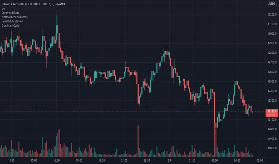
Volatility Percentile🎲 Volatility is an important measure to be included in trading plan and strategy. Strategies have varied outcome based on volatility of the instruments in hand.
For example,
🚩 Trend following strategies work better on low volatility instruments and reversal patterns work better in high volatility instruments. It is also important for us to understand the median volatility of an instrument before applying particular strategy strategy on them.
🚩 Different instrument will have different volatility range. For instance crypto currencies have higher volatility whereas major currency pairs have lower volatility with respect to their price. It is also important for us to understand if the current volatility of the instrument is relatively higher or lower based on the historical values.
This indicator is created to study and understand more about volatility of the instruments.
⬜ Process
▶ Volatility metric used here is ATR as percentage of price. Other things such as bollinger bandwidth etc can also be used with few changes.
▶ We use array based counters to count ATR values in different range. For example, if we are measuring ATR range based on precision 2, we will use array containing 10000 values all initially set to 0 which act as 10000 buckets to hold counters of different range. But, based on the ATR percentage range, they will be incremented. Let's say, if atr percent is 2, then 200th element of the array is increased by 1.
▶ When we do this for every bar, we have array of counters which has the division on how many bars had what range of atr percent.
▶ Using this array, we can calculate how many bars had atr percent more than current value, how many had less than current value, and how many bars in history has same atr percent as current value.
▶ With these information, we can calculate the percentile of atr percentage value. We can also plot a detailed table mentioning what percentile each range map to.
⬜ Settings
▶ ATR Parameters - this include Moving average type and Length for atr calculation.
▶ Rounding type refers to rounding ATR percentage value before we put into certain bucket. For example, if ATR percentage 2.7, round or ceil will make it 3, whereas floor will make it 2 which may fall into different buckets based on the precision selected.
▶ Precision refers to how much detailed the range should be. If precision set to 0, then we get array of 100 to collect the range where each value will represent a range of 1%. Similarly precision of 1 will lead to array of 1000 with each item representing range of 0.1. Default value used is 2 which is also the max precision possible in this script. This means, we use array of 10000 to track the range and percentile of the ATR.
▶ Display Settings - Inverse when applied track percentile with respect to lowest value of ATR instead of high. By default this is set to false. Other two options allow users to enable stats table. When detailed stats are enabled, ATR Percentile as plot is hidden.
▶ Table Settings - Allows users to select set size and coloring options.
▶ Indicator Time Window - Allow users to select particular timeframe instead of all available bars to run the study. By default windows are disabled. Users can chose start and end time individually.
Indicator display components can be described as below:

TASC 2021.12 Directional Movement w/Hann█ OVERVIEW
Presented here is code for the "Directional Movement w/Hann" indicator originally conceived by John Ehlers. The code is also published in the December 2021 issue of Trader's Tips by Technical Analysis of Stocks & Commodities (TASC) magazine.
Ehlers continues here his exploration of the application of Hann windowing to conventional trading indicators.
█ FEATURES
The rolling length can be modified in the script's inputs, as well as the width of the line.
█ NOTES
Calculations
The calculation starts with the classic definition of PlusDM and MinusDM. These directional movements are summed in an exponential moving average (EMA). Then, this EMA is further smoothed in a finite impulse response (FIR) filter using Hann window coefficients over the calculation period.
Background
The DMI and ADX indicators were designed by J. Welles Wilder and presented in his "New Concepts in Technical Trading Systems" book published in 1978.
Join TradingView!
