UM VIX30/VIX Regime & Volatility Roll Yield
SUMMARY
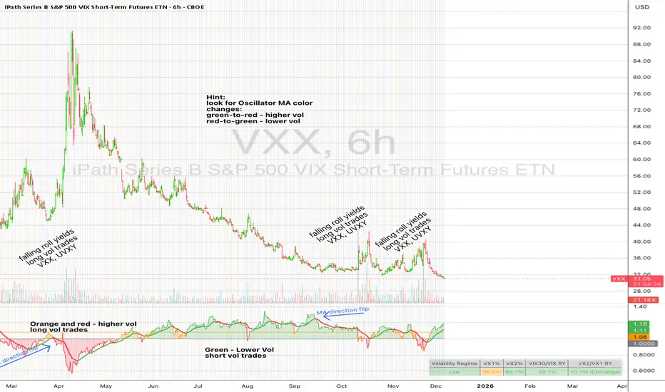
A front-of-the-curve volatility indicator that compares spot VIX to a synthetic 30-day VIX (VIX30) built from VX1/VX2 futures, revealing early volatility pressure, regime shifts, and roll-yield transitions. Ideal for timing long/short volatility trades in VXX, UVXY, SVIX, and VIX futures.
DESCRIPTION
This indicator compares spot VIX to a synthetic 30-day constant-maturity volatility estimate (“VIX30”) built from VX1 and VX2 futures. The VIX30/VIX Ratio reveals short-term volatility pressure and regime shifts that traditional VX1/VX2 roll-yield alone often misses.
VIX30 is constructed using true calendar-day interpolation between VX1 and VX2, with VX1% and VX2% showing the real-time weights behind the 30-day volatility anchor. The table displays the volatility regime, the VX1/VX2 weights, spot-term roll yield (VIX30/VIX), and futures-term roll yield (VX2/VX1), giving a complete, front-of-the-curve perspective on volatility dynamics.
Use this to spot early volatility expansions, collapsing contango, and regime transitions that influence VXX, UVXY, SVIX, VX options, and VIX futures.
HOW IT WORKS
The script calculates the exact calendar days to expiration for the front two VIX futures. It then applies linear interpolation to blend VX1 and VX2 into a 30-day constant-maturity synthetic volatility measure (“VIX30”). Comparing VIX30 to spot VIX produces the VIX30/VIX Ratio, which highlights short-term volatility pressure and regime direction. A full term-structure table summarizes regime, VX1%/VX2% weights, and both spot-term and futures-term roll yields.
DEFAULT SETTINGS
VX1! and VX2! are used by default for front-month and second-month futures. These may be manually overridden if TradingView rolls contracts early. The default timeframe is 30 minutes, and the VIX30/VIX Ratio uses a 21-period EMA for regime smoothing. The historical threshold is set to 1.08, reflecting the long-run average relationship between VIX30 and VIX.
SUGGESTED USES
• Identify early volatility expansions before they appear in VX1/VX2 roll yield.
• Confirm contango/backwardation shifts with front-of-curve context.
• Time long/short volatility trades in VXX, UVXY, SVIX, and VX options.
• Monitor regime transitions (Low → Cautionary → High) to anticipate trend inflections.
• Combine with price action, Nadaraya-Watson trends, or MA color-flip systems for higher-confidence entries.
• MA red → green flips may signal opportunities to short volatility or increase equity exposure.
• MA green → red flips may signal opportunities to go long volatility, reduce equity exposure, or take short-equity positions.
ALERTS
Alerts trigger when the ratio crosses above or below the historical threshold or when the moving-average slope flips direction. A green flip signals rising volatility pressure; a red flip signals fading or collapsing volatility. These alert conditions can be used to automate long/short volatility bias shifts or trade-entry notifications.
FURTHER HINTS
• Increasing orange/red in the table suggests an emerging higher-volatility environment.
• SVIX (inverse volatility ETF) can trend strongly when volatility decays; on a 6-hour chart, MA green flips often align with attractive short-volatility opportunities.
• For long-volatility trades, consider shrinking to a 30-minute chart and watching for MA green → red flips as early entry cues.
• Experiment with different timeframes and smoothing lengths to match your trading style.
• Higher VIX30/VIX and VX2/VX1 roll yields generally imply faster decay in VXX, UVXY, and UVIX — or stronger upside momentum in SVIX.
• The author likes the 6-hour chart for short vol, and the 30-minute chart for long vol. Long vol trades are fast and furious so you want to be quick.
תנודתיות
SigmaFrame-FESXSigmaFrame is a volatility-weighted standard deviation engine designed to generate dynamic intraday pivot levels which expand during volatility spikes and tighten during compression, giving traders a consistent structural map across trending and rotational environments.

Institutional VWAP Suite (Lite Compatible)The **Institutional VWAP Suite (Lite Compatible)** brings true institutional volume-weighted price analysis to every trader — even on TradingView Lite/Free accounts where standard VWAP tools are restricted.
This script recreates the most important VWAP models used by banks, funds, and high-frequency desks, including:
• **Daily VWAP** (exchange-accurate)
• **Weekly VWAP** (manually accumulated)
• **Monthly VWAP** (manually accumulated)
• **Rolling Window VWAP** (array-based, fully Lite-compatible)
All calculations avoid blocked functions like `ta.sum` or session-restricted VWAP calls. Everything is built manually from volume and price to ensure accuracy across all accounts and all markets.
### Features
• Multi-timeframe VWAPs (Daily/Weekly/Monthly)
• Manual Rolling VWAP with adjustable length
• Optional VWAP bands (Lite-safe)
• Clean visuals with color-coded levels
• Optimized arrays for fast, stable performance
• Free-tier compatible — no premium functions required
This tool is designed for traders who want institutional structure, premium-level VWAP calculations, and consistent execution regardless of plan level. Perfect for scalpers, day traders, futures traders, and anyone who uses intraday volume profiles.
### Recommended Use
• Map directional bias using Daily vs Weekly VWAP
• Use Monthly VWAP for macro trend context
• Track intraday mean reversion with Rolling VWAP
• Use VWAP bands as dynamic support/resistance zones
A simple, powerful, no-restrictions VWAP engine — built for everyone.

Open Interest Delta AggregateOpen Interest Delta - By Randy (Multi-Exchange Version)This Pine Script indicator calculates and displays the daily change (delta) in total Open Interest across multiple major perpetual futures exchanges.Key Features:Aggregates Open Interest from Binance, OKX, ByBit, Bitget, HTX, and the current chart’s exchange (if any).
You toggle each exchange on/off individually — it automatically sums all active sources.
Plots OI Delta as histogram columns (Type 1 = combined, Type 2 = separate positive/negative).
Uses dynamic thresholds based on standard deviation of positive/negative OI delta EMA to classify changes as:Normal (yellow)
Medium (orange)
Large (red)
Extreme (purple)
Optionally colors price candles when OI delta crosses these significant thresholds (great for spotting big money moves).
Works best on daily timeframe (automatically switches to daily OI data even if you're viewing lower timeframes).
In Simple Terms:It shows you when huge amounts of new positions (long or short) are being opened across the biggest crypto futures exchanges — a powerful signal of institutional/smart money activity and potential trend strength or reversals. The more exchanges light up with extreme OI delta, the stronger the conviction behind the move.

Hierarchical Hidden Markov Model - Probability Cone
The Hierarchical Hidden Markov Model - Probability Cone Indicator employs Hierarchical Hidden Markov Models for forecasting future price movements in financial markets. HHMMs are statistical tools that predict transitions between hidden states, such as different market regimes, based on observed data. This makes them valuable for understanding market behaviours and projecting future price trajectories. As discussed in the Hierarchical Hidden Markov Model indicator, HHMMs predict future states and their associated outputs based on the current state and model parameters. This tool is fundamentally very similar to the traditional HMM . The application of the HHMM for generating a probability cone forecast is therefore also fundamentally the same between HMM and HHMM. Despite their significant similarity I will go through the same fundamental examples of how probability cone is generated for the HHMM as I did for the HMM probability cone .
As you might know by now the probability cone indicator uses the knowledge about the current identified "state" or "regime" and with the help of transition probabilities, emission probabilities and initial probabilities generate a probabilistic forecast of the expected future price movements. To better understand the behind the Probability Cone we encourage you to use and learn about our free version of the Probability Cone as well as for even deeper understanding the Probability Cone Pro.
WHAT ARE REGIME DEPENDENT FORECASTS
We established that the indicator creates probabilistic forecasts of future price movements dependent on the current identified "state" or market "regime" via the Hidden Markov Model. In the image below we can see an example.
In this example we can see 4 different probability cones forecasting a 70% and 90% probability range (15% and 5% quantiles respectively). What you may notice is that the 4 probability cones look vastly different, despite using the same probability ranges as well as being generated from the same model trained on virtually the same data. What allows for this difference in the forecast, is conditioning the forecast on the current most likely identified state by the HHMM.
The first most cone is generating a forecast taking into account that the model identified the current market condition to be a extremely low in volatility this is a characteristic of the state identified by the light green coloured posterior probability. The second cone is significantly wider as well as has a negative drift, this is the case because that state identified by the red posterior probability is characterised by the most extreme volatility along with significant negative returns. The cone after that remains quite wide however is again associated with positive returns, this is characteristic of the state that the model identified via a high yelow coloured posterior probability. The last probability cone is again generated from a state that is characterised by quite low volatility albeit not the lowest. We can also see the state associated with that behaviour is identified by the high dark green posterior probability which is the highest at that time.
NOTE! Those are within sample forecasts, you can find more information on the difference between within sample model fit and out of sample prediction in the HHMM indicator description
This indicator also allows you to specify whether you wish to display probability based labels at the edges of the cone or whether you would prefer to display percent change based labels. With percent change labels you get the exact percentage value of the probabilistic increase or decrease of the price. See the example below
BARS BACK OFFSET vs DATE BASED OFFSET
The cones position can be offset by specifying the number of bars we wish to move it back similarly as with the rest of probability cone indicators. This indicator has however an additional, date based offset implemented. A user can therefore specify the position of the cone by specifying a date in the settings. The advantage of using the date based offset is that once it is turned on the user can also slide the cone up and down the chart with their mouse without having to manually adjust the date in the settings.
DIFFICULTIES WITH GENERATING FORECASTS (advanced):
The estimation of the probability cone, gets more difficult the more complex the model gets. A simple normal distribution probability cone can scale the distribution over time by simply multiplying the drift by the number of time steps and the volatility by the square root of time steps we wish to forecast for. More complex distributions often have to rely on mode advanced methods like convolutions, monte carlo or other kinds of approximations.
To estimate the probability cone forecast for the Hierarchial Hidden Markov Model, the indicator integrates two primary methodologies: Gaussian approximation and importance sampling. The Gaussian approximation is utilised for estimating the central 90% of future prices. This method provides a quick and efficient estimation within this central range, capturing the most likely price movements. The gaussian approximation will result in a forecast with an equal mean and variance as the true forecast, it will however not accurately reflect higher moments like skewness and kurtosis. For that reason the tail quantiles, which represent extreme price movements beyond the central range (90%), are estimated via importance sampling. This approach ensures a more accurate estimation of the skewness and kurtosis associated with extreme scenarios. While importance sampling leverages the flexibility of Monte Carlo as well as attempts to increase its efficiency by sampling from more precise areas of the distribution, the importance sampling may still underestimate most extreme quantiles associated with the lowest probabilities which is an inherent limitation of the indicator.
Example of gaussian approximation cone for probabilities above 5% (90% range):
Example of importance sampling cone for tail probabilities lower than 5% (beyond 90% range):
WARNING!
As per usual understand that the probabilities are estimations and best guesses based on the historical data and the patterns identified by the model and do not represent the true probability which is unknown in reality.
Settings:
- Source: Data source used for the model
- Forecast Period: Number of bars ahead for generating forecasts.
- Simulation Number: Number of Monte Carlo simulations to run in the case of importance sampling
-Body Probability: Specifies the inner range of the probability cone. The probability specifies the ammount of observations that are expected to fall outside of this range
- Tail Probability: Specifies the outter range of the probability cone. When this probability is under 5%, importance sampling will turn on
- Lock Cone: When ticked on, the cone will be locked at its current position.
- Offset Cone Based on Date: When ticked on, the position of the cone will be determined by the selected date.
- Offset: When "Offset Cone Based on Date" is turned off, you can use offset setting to specify the position of the cone projection.
- Date: When "Offset Cone Based on Date" is turned on, you can use the date setting to specify the date from which the forecast starts.
- Reestimate Model Every N Bars: This is especially useful if you wish to use the indicator on lower timeframes where model estimation might take longer than for the new datapoint to arrive. In that case you can specify after how many bars the model should be reestimated.
- Training Period: Length of historical data used to train the HMM.
- Expectation Maximization Iterations: Number of iterations for the EM algorithm.
- Cone Colors: Customizable colors for the probability cone, when approximation is on and when importance sampling is on

Hidden Markov Model - Probability Cone
The Hidden Markov Model - Probability Cone Indicator employs Hidden Markov Models (HMMs) for forecasting future price movements in financial markets. HMMs are statistical tools that predict transitions between hidden states, such as different market regimes, based on observed data. This makes them valuable for understanding market behaviours and projecting future price trajectories. As discussed in the Hidden Markov Model indicator, HMMs predict future states and their associated outputs based on the current state and model parameters.
The probability cone indicator therefore uses the knowledge about the current identified "state" or "regime" and with the help of transition probabilities, emission probabilities and initial probabilities generate a probabilistic forecast of the expected future price movements. To better understand the behind the Probability Cone we encourage you to use and learn about our free version of the Probability Cone as well as for even deeper understanding the Probability Cone Pro.
WHAT ARE REGIME DEPENDENT FORECASTS
As mentioned above the indicator creates probabilistic forecasts of future price movements dependent on the current identified "state" or market "regime" via the Hidden Markov Model. In the image below we can see an example.
In this example we can see 3 different probability cones forecasting a 70% and 90% probability range (15% and 5% quantiles respectively). What you may notice is that the 3 probability cones look vastly different, despite using the same probability ranges as well as being generated from the same model trained on virtually the same data. What allows for this difference in the forecast is conditioning the forecast on the current most likely identified state by the HMM.
The first most wide cone is generating a forecast taking into account that the model identified the current market condition to be a very volatile which is a characteristic of the state identified by the orange coloured posterior probability. The second cone is significantly more narrow as that state identified by the purple posterior probability is characterised by lower volatility. Nevertheless, the last probability cone is generated from the state that is characterised by the lowest volatility, we can also see the light blue posterior probability to be the highest at that time.
The indicator also allows you to specify whether you wish to display probability based labels at the edges of the cone or whether you would prefer to display percent change based labels. With percent change labels you get the exact percentage value of the probabilistic increase or decrease of the price. See the example below
BARS BACK OFFSET vs DATE BASED OFFSET
The cones position can be offset by specifying the number of bars we wish to move it back similarly as with the rest of probability cone indicators. This indicator has however an additional, date based offset implemented. A user can therefore specify the position of the cone by specifying a date in the settings. The advantage of using the date based offset is that once it is turned on the user can also slide the cone up and down the chart with their mouse without having to manually adjust the date in the settings.
DIFFICULTIES WITH GENERATING FORECASTS (advanced):
The estimation of the probability cone, gets more difficult the more complex the model gets. A simple normal distribution probability cone can scale the distribution over time by simply multiplying the drift by the number of time steps and the volatility by the square root of time steps we wish to forecast for. More complex distributions often have to rely on mode advanced methods like convolutions, monte carlo or other kinds of approximations.
To estimate the probability cone forecast for the Hidden Markov Model, the indicator integrates two primary methodologies: Gaussian approximation and importance sampling. The Gaussian approximation is utilized for estimating the central 90% of future prices. This method provides a quick and efficient estimation within this central range, capturing the most likely price movements. The gaussian approximation will result in a forecast with an equal mean and variance as the true forecast, it will however not accurately reflect higher moments like skewness and kurtosis. For that reason the tail quantiles, which represent extreme price movements beyond the central range (90%), are estimated via importance sampling. This approach ensures a more accurate estimation of the skewness and kurtosis associated with extreme scenarios. While impoortance sampling leverages the flexibility of monte carlo as well as attempts to increase its efficiency by sampling from more precise areas of the distribution, the importance sampling may still underestimate most extreme quantiles associated with the lowest probabilties which is an inherent limitation of the indicator.
Example of gaussian approximation cone for probabilities above 5% (90% range):
Example of importance sampling cone for tail probabilities lower than 5% (beyond 90% range):
WARNING!
As per usual understand that the probabilities are estimations and best guesses based on the historical data and the patterns identified by the model and do not represent the true probability which is unknown in reality.
Settings:
- Source: Data source used for the model
- Forecast Period: Number of bars ahead for generating forecasts.
- Simulation Number: Number of Monte Carlo simulations to run in the case of importance sampling
-Body Probability: Specifies the inner range of the probability cone. The probability specifies the ammount of observations that are expected to fall outside of this range
- Tail Probability: Specifies the outter range of the probability cone. When this probability is under 5%, importance sampling will turn on
- Lock Cone: When ticked on, the cone will be locked at its current position.
- Offset Cone Based on Date: When ticked on, the position of the cone will be determined by the selected date.
- Offset: When "Offset Cone Based on Date" is turned off, you can use offset setting to specify the position of the cone projection.
- Date: When "Offset Cone Based on Date" is turned on, you can use the date setting to specify the date from which the forecast starts.
- Reestimate Model Every N Bars: This is especially useful if you wish to use the indicator on lower timeframes where model estimation might take longer than for the new datapoint to arrive. In that case you can specify after how many bars the model should be reestimated.
- Training Period: Length of historical data used to train the HMM.
- Expectation Maximization Iterations: Number of iterations for the EM algorithm.
- Cone Colors: Customizable colors for the probability cone, when approximation is on and when importance sampling is on

ARCH ProxyARCH Proxy (ARCH) - Volatility Assessment Indicator
The ARCH Proxy indicator (short title: ARCH) is a dynamic, multi-factor volatility assessment tool designed to help traders quickly gauge the current energy and risk level of the market. It plots a real-time measure of price fluctuation against its long-term historical average and adaptive High/Low Volatility thresholds. This provides a clear, objective framework for distinguishing between periods of market compression (low-energy consolidation) and expansion (high-risk volatility), optimizing strategy selection and risk management.
Simplified Trading Guide
The ARCH indicator offers a clear, objective signal framework to guide your trading decisions based on market energy :
Spotting High-Risk Expansion (Climax):
Signal: The main ARCH Proxy line moves sharply above the High Volatility Threshold (typically a red line).
Action: This signals the market is in a period of intense, climactic price action. This is often a time to avoid new entries, reduce exposure, or look for potential trend exhaustion and reversals due to the high risk of a sudden correction.
Identifying Low-Energy Compression (Setup):
Signal: The main ARCH Proxy line trends consistently below the Low Volatility Threshold (typically a green line).
Action: This indicates a market consolidation phase. This "low-energy" compression frequently precedes a strong breakout (expansion). Traders should prepare for an entry in the direction of the dominant trend, anticipating a coming surge in momentum.
Normal Trading Conditions:
Signal: The ARCH Proxy line is fluctuating between the High and Low Volatility thresholds.
Action: The market is in a normal state. Use this time to follow the dominant trend with standard risk parameters.

Watermark | Bar Time | Average Daily RangeMulti Info Panel & Watermark
Multi Info Panel & Watermark is a utility indicator that displays several pieces of chart information in a single, customizable panel. It is designed to support intraday and swing analysis by making key data—such as symbol details, date, and average daily range—easy to see at a glance, as well as providing simple tools for notes and backtesting.
Features
Watermark / Custom Note
Optional text overlay that can be used as a watermark or personal note.
Can display a strategy name, reminder, or any other user-defined label on the chart.
Ticker Info
Shows information about the currently active symbol on the chart (for example, symbol name and other basic details depending on the inputs).
Helps keep track of which market or pair is being analyzed, especially when using multiple charts.
Current Date
Displays the current date directly on the chart.
Useful for screenshots, journaling, and documenting analysis.
Average Daily Range (ADR)
Calculates the average daily range of the active symbol over a user-defined number of recent days.
Helps visualize how much price typically moves in a day, which can support position sizing, target setting, or volatility awareness within your own trading approach.
Open Bar Time Marker
Marks the open time of a selected bar (for example, a session open or a specific reference bar).
Primarily intended as a visual aid for manual backtesting and reviewing historical price action.
Usage
Use the watermark and ticker info to keep your charts labeled and organized.
Refer to the ADR readout to understand typical daily volatility of the instrument you are studying.
Use the date and open bar time marker when creating screenshots, trade journals, or when replaying historical sessions for review.
This script does not generate trading signals and does not guarantee any performance or results. It is provided solely as an informational and visualization tool. Always combine it with your own analysis, risk management, and decision-making. Nothing in this indicator or description should be considered financial advice.

Force Pulse█ OVERVIEW
Force Pulse is a fast-reacting oscillator that measures the internal strength of market sides by analyzing the aggregated dominance of bulls and bears based on candle size.
The indicator normalizes this difference into a 0–100 range, generates signals (OB/OS, midline cross, MA midline cross), and detects divergences between price and the oscillator.
It also offers advanced visualization, signal markers, and alerts, making it a versatile tool suitable for many trading styles.
█ CONCEPTS
Force Pulse was designed as a universal tool that can be applied to various trading strategies depending on its settings:
- increasing the period lengths and smoothing transforms it into a momentum/trend indicator, revealing a stable dominance of one market side.
- Lowering these parameters turns it into a peak/low detector, ideal for contrarian and mean-reversion strategies.
The oscillator analyzes the relationship between the sum of bullish and bearish candles over a selected period, based on:
- candle body size, or
- average candle body size (AVG Body).
Depending on the selected mode, OB/OS levels should be adjusted, as value dynamics differ between modes.
The output is normalized to 0–100, where:
> 50 – bullish dominance,
< 50 – bearish dominance.
The additional MA line is derived from smoothed oscillator values and serves as a signal line for midline crosses and as a trend filter.
The indicator also detects divergences (HL/LL) between price and the oscillator.
█ FEATURES
Bull & Bear Strength:
- Calculations are based on Body or AVG Body – mode selection requires adjusting OB/OS levels.
- Bullish and bearish candle values are summed separately.
- All results are normalized to the 0–100 scale.
Force Pulse Oscillator:
- The main line reflects the current dominance of either market side.
Dynamic colors:
- Green – above 50,
- Red – below 50.
Signal MA:
- SMA based on oscillator values functions as a signal line.
- Helps detect momentum shifts and generates signals via midline crosses.
- Can serve as a trend confirmation filter.
Overbought / Oversold:
- Configurable OB/OS levels, also for the MA line.
- Dynamic OB/OS line colors: when the MA line exceeds the defined threshold (e.g., MA > maOverbought or MA < maOversold), OB/OS lines change color (red/green).
- This often signals a potential reversal or correction and may act as additional confirmation for oscillator-generated signals.
Divergences:
- Detection based on swing pivots:
- Bullish: price LL, oscillator HL
- Bearish: price HH, oscillator LH
- Displayed as “Bull” / “Bear” labels.
Signals:
Supports multiple signal types:
- Overbought/Oversold Cross
- Midline Cross
- MA Midline Cross (based on the signal MA line)
- Signals appear as triangles above/below the oscillator.
Visualization:
- Gradient options for lines and levels.
- Full customization of colors, transparency, and line thickness.
Alerts available for:
- Divergences
- OB/OS crossings
- Midline crossings
- MA midline crossings
█ HOW TO USE
Add the indicator to your TradingView chart → Indicators → search “Force Pulse”
Parameter Configuration
Calculation Settings:
- Calculation Period (lookback) – defines the strength calculation window.
Force Mode (Body / AVG Body):
- Body – faster response, higher sensitivity.
- AVG Body – more stable output; adjust band levels and periods to your strategy.
- EMA Smoothing (smoothLen) – reduces oscillator noise.
- MA Length – length of the signal line (SMA).
Threshold Levels:
- Set Overbought/Oversold levels for both the oscillator and the MA line.
- Adjust levels depending on Body / AVG Body mode.
Divergence Detection:
- Enable/disable divergence detection.
- PivotLength affects both delay and signal quality.
- Signal Settings: Choose one or multiple signal types.
- Style & Colors: Full control over color schemes, gradients, and transparency.
Signal Interpretation
BUY:
- Oscillator leaves oversold (OS crossover).
- Midline cross upward.
- MA crosses the midline from below.
- Bullish divergence.
SELL:
- Oscillator leaves overbought (drops below OB).
- Midline cross downward.
- MA crosses the midline from above.
- Bearish divergence.
Trend / Momentum:
-Longer periods and stronger smoothing → stable directional signals.
-MA as a trend filter: e.g., signal line above the midline (50) and MA pointing upward indicates continuation of a bullish impulse.
Contrarian / Mean Reversion:
- Short periods → rapid detection of peaks and troughs; ideal for contrarian signals and pullback entries.
█ APPLICATIONS
- Trend Trading: Using midline and MA midline crosses to determine direction.
- Reversal Trading: OB/OS levels and divergences help identify reversals.
- Scalping & Intraday: Short settings + signal line above the midline with bullish MA → shows short-term impulse and continuation.
- Swing Trading: Longer MA and higher lookback provide a stable view of market-side dominance.
- Momentum Analysis: Force Pulse highlights the strength of the wave before price movement occurs.
█ NOTES
- In strong trends, the oscillator may stay in extreme zones for a long time — this reflects dominance, not necessarily a reversal signal.
- Divergences are more reliable on higher timeframes.
- OB/OS levels should be tailored to Body/AVG Body mode and the instrument.
- Best results come from combining the indicator with other tools (S/R, market structure, volume).

Probability Cone ProProbability Cone Pro is based on the Expected Move Pro . While Expected Move only shows the historical value band on every bar, probability cone extend the period in the future and plot a cone or curve shape of the probable range. It plots the range from bar 1 all the way to any specified number of bars up to 1000.
Probability Cone Pro is an upgraded version of the Probability Cone indicator that uses a Normal Distribution to model the returns. This newer version uses a maximum likelihood estimation for Asymmetric Laplace distribution parameters. Asymmetric Laplace distribution takes into account fatter tails and volatility clustering during low volatility. So it will be thinner in the body (eg: <70% range) and fatter in the tails (>95% range) which fits the stock return better. Despite a better fit users should not blindly follow the probabilities derived from the indicator and should understand that these are very precise estimations of probability based on historical data, not the true probability which is in reality unknown.
When we compare the more peaked asymmetric laplace to the bell curve shaped normal distribution we can see that the asymmetric laplace fits the empirical data (blue histogram) significantly better. The fit is improved in both the body (middle peaked part) as well as in the fatter tails (more of extreme occurrences far from the center)
The area of probability range is based on an inverse cumulative distribution function. The inverse cumulative distribution gives the range of price for given input probability. People can adjust the range by adjusting the input probability in the settings. The entered probability will be shown at the edges of the cone when the “show probability” setting is on.
The indicator allows for specifying the probability for 2 quantiles on each side of the distribution , therefore 4 distinct probability values. The exact probability input is another distinction compared to the Normal Distribution based Probability Cone, in which the probability range is determined by the input of a standard deviation. Additionally now the displayed labels at the edges of the probability cone no longer correspond to the total number of outcomes that are expected to occur within the specific range, instead we chose to display the inverse which is the probability of outcomes outside of the specified range. See comparison below:
Probability cone pro with 68% and 95% ranges also defined by 16% and 2.5% probabilities at the tails on both sides:
Normal Probability cone with 68% and 95% ranges defined by 1st and 2nd standard deviation
SETTINGS:
Bars Back : Number of bars the cone is offset by.
Forecast Bar: Number of bars we forecast the cone for in the future.
Lock Cone : Specify whether we wish t lock the cone to the current bar, so it does not move when new bars arrive.
Show Probability : Specify whether you wish to show the probability labels at the edges of the cone.
Source : Source for computation of log returns whose distribution we forecast
Drift : Whether to take into account the drift in returns or assume 0 mean for the distribution.
Period: The sampling period or lookback for both the drift and the volatility estimation (full distribution estimation).
Up/Down Probabilities: 4 distinct probabilities are specified, 2 for the upper and 2 for the lower side of the distribution.

Expected Move ProExpected Move is the amount that an asset is predicted to increase or decrease from its current price, based on the current levels of volatility.
This Expected Move Pro indicator uses a maximum likelihood estimation for Asymmetric Laplace distribution parameters, and is an upgrade from the regular Expected Move indicator that uses a Normal Distribution. The use of the Asymmetric Laplace distribution ensures a probability range more accurate than the more common expected moves based on a normal distribution assumption for returns. Asymmetric Laplace distribution takes in account fatter tails and volatility clustering during low volatility. So it will be thinner in the body (eg: <70% range) and fatter in the tails (>95% range) which fits the stock return better.
When we compare the more peaked asymmetric laplace to the bell curve shaped normal distribution we can see that the asymmetric laplace fits the empirical data (blue histogram) significantly better. The fit is improved in both the body (middle peaked part) as well as in the fatter tails (more of extreme occurrences far from the center)
EXPECTED MOVE PROBABILITY:
In the expected move settings, the user can specify the range probability they wish to display. In a normal distribution a 1 standard deviation range corresponds to a range within which just under 70% of observations fall. So to specify a 70% probability range one would set 15% probability for both the upper and lower range.
For the more extreme ranges a two tail function is used so the user can only specify one probability. When 5% probability is specified the range will cover 95% and on each side of the range the probability of an occurence that extreme will be 2.5%. In the above Image we can see two tail probabilities specified at 5% and 1%, covering the 95% and 99% ranges respectively.
The indicator also allows for multi timeframe usecases. One can request a daily or perhaps even weekly expected move on an hourly chart, like we see below.
SETTINGS:
Resolution: Specify the timeframe and if you want to use the multi timeframe functionality.
Real Time : Do you wish the expected move to adjust with the current open price or do you wish it to be a forecast based on the yesterdays close. If latter, keep it OFF.
Sample Size : Lookback or the number of bars we sample in the calculation.
Optimization : Keep it on for speed purposes, only slightly higher precision will be achieved without optimization.
Probabilities: One tail - left and right, specify probability for each side of the range, two tail - single probability split in half for each side of the range
Center : Displays the central line which is the central tendency of a distribution / the median
Hide History : Hides expected moves and only the expected move for the current bar remains.
Plot Style Settings : One can adjust the line styles, box styles as well as width and transparency.

Probability Cone█ Overview:
Probability Cone is based on the Expected Move . While Expected Move only shows the historical value band on every bar, probability panel extend the period in the future and plot a cone or curve shape of the probable range. It plots the range from bar 1 all the way to bar 31.
In this model, we assume asset price follows a log-normal distribution and the log return follows a normal distribution.
Note: Normal distribution is just an assumption; it's not the real distribution of return.
The area of probability range is based on an inverse normal cumulative distribution function. The inverse cumulative distribution gives the range of price for given input probability. People can adjust the range by adjusting the standard deviation in the settings. The probability of the entered standard deviation will be shown at the edges of the probability cone.
The shown 68% and 95% probabilities correspond to the full range between the two blue lines of the cone (68%) and the two purple lines of the cone (95%). The probabilities suggest the % of outcomes or data that are expected to lie within this range. It does not suggest the probability of reaching those price levels.
Note: All these probabilities are based on the normal distribution assumption for returns. It's the estimated probability, not the actual probability.
█ Volatility Models :
Sample SD : traditional sample standard deviation, most commonly used, use (n-1) period to adjust the bias
Parkinson : Uses High/ Low to estimate volatility, assumes continuous no gap, zero mean no drift, 5 times more efficient than Close to Close
Garman Klass : Uses OHLC volatility, zero drift, no jumps, about 7 times more efficient
Yangzhang Garman Klass Extension : Added jump calculation in Garman Klass, has the same value as Garman Klass on markets with no gaps.
about 8 x efficient
Rogers : Uses OHLC, Assume non-zero mean volatility, handles drift, does not handle jump 8 x efficient.
EWMA : Exponentially Weighted Volatility. Weight recently volatility more, more reactive volatility better in taking account of volatility autocorrelation and cluster.
YangZhang : Uses OHLC, combines Rogers and Garmand Klass, handles both drift and jump, 14 times efficient, alpha is the constant to weight rogers volatility to minimize variance.
Median absolute deviation : It's a more direct way of measuring volatility. It measures volatility without using Standard deviation. The MAD used here is adjusted to be an unbiased estimator.
You can learn more about each of the volatility models in out Historical Volatility Estimators indicator.
█ How to use
Volatility Period is the sample size for variance estimation. A longer period makes the estimation range more stable less reactive to recent price. Distribution is more significant on larger sample size. A short period makes the range more responsive to recent price. Might be better for high volatility clusters.
People usually assume the mean of returns to be zero. To be more accurate, we can consider the drift in price from calculating the geometric mean of returns. Drift happens in the long run, so short lookback periods are not recommended.
The shape of the cone will be skewed and have a directional bias when the length of mean is short. It might be more adaptive to the current price or trend, but more accurate estimation should use a longer period for the mean.
Using a short look back for mean will make the cone having a directional bias.
When we are estimating the future range for time > 1, we typically assume constant volatility and the returns to be independent and identically distributed. We scale the volatility in term of time to get future range. However, when there's autocorrelation in returns( when returns are not independent), the assumption fails to take account of this effect. Volatility scaled with autocorrelation is required when returns are not iid. We use an AR(1) model to scale the first-order autocorrelation to adjust the effect. Returns typically don't have significant autocorrelation. Adjustment for autocorrelation is not usually needed. A long length is recommended in Autocorrelation calculation.
Note: The significance of autocorrelation can be checked on an ACF indicator.
ACF
Time back settings shift the estimation period back by the input number. It's the origin of when the probability cone start to estimation it's range.
E.g., When time back = 5, the probability cone start its prediction interval estimation from 5 bars ago. So for time back = 5 , it estimates the probability range from 5 bars ago to X number of bars in the future, specified by the Forecast Period (max 1000).
█ Warnings:
People should not blindly trust the probability. They should be aware of the risk evolves by using the normal distribution assumption. The real return has skewness and high kurtosis. While skewness is not very significant, the high kurtosis should be noticed. The Real returns have much fatter tails than the normal distribution, which also makes the peak higher. This property makes the tail ranges such as range more than 2SD highly underestimate the actual range and the body such as 1 SD slightly overestimate the actual range. For ranges more than 2SD, people shouldn't trust them. They should beware of extreme events in the tails.
The uncertainty in future bars makes the range wider. The overestimate effect of the body is partly neutralized when it's extended to future bars. We encourage people who use this indicator to further investigate the Historical Volatility Estimators , Fast Autocorrelation Estimator , Expected Move and especially the Linear Moments Indicator .
The probability is only for the closing price, not wicks. It only estimates the probability of the price closing at this level, not in between.

WSMR v3.9 — WhaleSplash → Mean Reversal
# WSMR v3.9 — WhaleSplash → Mean Reversal
*A Non-Repainting Impulse‑Reversal Engine for Systematic Futures Trading*
## Overview
WSMR v3.9 is a complete impulse → exhaustion → mean‑reversion framework designed for systematic intraday trading. It identifies high‑energy displacement events (“WhaleSplashes”), measures volatility structure, tracks VWAP deviation, and confirms reversals using RSI divergence, Z‑Score resets, SMA20 reclaim, and pivot-based structure.
All signals are non‑repainting and alerts fire on bar close.
---
## Core Components
### 1. WhaleSplash (Short Impulse Event)
Triggered when a candle meets displacement conditions:
- Large bar range vs ATR
- Minimum % move
- Volume expansion
- VWAP deviation (tick-based)
- Z‑Score oversold / RSI exhaustion
- Volatility-gated
### 2. Mean Reversal Long (MR)
Requires:
- RSI bullish divergence
- Z‑Score reset
- SMA20 reclaim
- Higher-low confirmation
### 3. First-Candle Confirmation (Optional)
- MR Confirm → first green after MR
- WS Confirm → first red after WS
- TTL window configurable
### 4. Asia Session Filter
Optional restriction to:
**23:00 → 09:00 UTC**
### 5. Volatility Monitor
Detects:
- Normal
- Wicky
- Spiky
- Extreme
### 6. WS Frequency Analytics
Rolling frequency calculation across:
- Bars / Days / Weeks / Months
---
## Status Panel (Top-Right)
Shows:
- Mode (Global / Asia-only)
- Timeframe + TTL
- WS frequency
- Volatility state
---
## Alerts
- WhaleSplash SHORT
- WhaleSplash LONG (MR)
- MR Confirm LONG
- WS Confirm SHORT
- Volatility Warning
---
## Notes
- Fully non‑repainting
- Stable bar-close logic
- Optimised for 1m–5m
- Works on futures, indices, metals, FX


RSI Cross Below 30 – Red Background StripShows red bars on chart in instances where RSI drops below 30

Book of Fish: Universal Deep DiveAhoy, Captain. 🏴☠️
Here is your official Angler’s Manual for the Book of Fish: Universal Deep Dive. This guide translates every pixel on your TradingView chart into nautical instruction so you can navigate the currents and land the big catch.
Print this out, tape it to your monitor, and respect the code of the sea.
________________________________________
📖 The Angler’s Manual: How to Fish
A Guide to the "Universal Deep Dive" Indicator
🌊 1. Check the Current (Background Color)
Before you cast a line, you must know which way the river is flowing.
• Green Water (Background): The tide is coming in. The broad market (Advancers) is beating the losers.
o The Rule: We prefer Longs (Calls). Swimming upstream against the green current is dangerous.
• Red Water (Background): The tide is going out. The market is heavy.
o The Rule: We prefer Shorts (Puts). Don't fight the gravity.
Captain’s Note: If your specific fish (stock) is Green while the water is Red, that’s a Monster Fish (Relative Strength). It’s strong, but keep a tight drag—if it gets tired, the current will drag it down fast.
________________________________________
🐟 2. Identify the Species (Candle Colors)
The color of your bars tells you exactly what strategy to deploy.
🟢 The Marlin (Ultra Bull)
• Visual: Green Candles. Price is riding above the Yellow Wave (20 EMA), and the Yellow Wave is above the White Whale (200 EMA).
• Strategy: Trend Following.
• How to Fish:
o Wait for the fish to swim down and touch the Yellow Wave.
o If it bounces? CAST! (Enter Long).
o Target: Let it run until the trend bends.
🔴 The Barracuda (Ultra Bear)
• Visual: Red Candles. Price is diving below the Yellow Wave, and the Yellow Wave is below the White Whale.
• Strategy: Trend Following (Short).
• How to Fish:
o Wait for the fish to jump up and hit the Yellow Wave.
o If it rejects? CAST! (Enter Short).
🟠 The Bottom Feeder (No Man’s Zone)
• Visual: Orange or Lime Candles. The price is fighting the trend (e.g., Price is below Yellow, but Yellow is still above White).
• Strategy: Reversion to Mean (Scalping).
• How to Fish:
o You are catching small fry here.
o Target: The Purple Anchor (VWAP) or the White Whale (200 EMA).
o Rule: As soon as it hits the Anchor or the Whale, cut the line and take your profit. Do not hold for a home run.
________________________________________
🎣 3. The Tackle Box (Signals & Icons)
These shapes are your triggers. They tell you when to strike.
Icon Name Meaning Action
▲ (Green Triangle) 3-Bar Play THE STRIKE. Momentum is breaking out after a rest. ENTER NOW. This is the sharpest hook in the box. Trend is resuming.
🔷 (Blue Diamond) Inside Bar The Nibble. Price is coiling/resting. Set a trap. Place a stop-entry slightly above the diamond (for longs).
⚫ (Black Dots) The Squeeze Calm Waters. Volatility has died. DO NOT CAST. Wait. When the dots disappear, the storm (and the move) begins.
9️⃣ (Red/Green Number) Exhaustion Full Net. The school has swum too far in one direction. Take Profits. A Red 9 at the top means the bull run is tired. A Green 9 at the bottom means the bear dive is ending.
✖️ (Purple Cross) RSI Snag Hazard. The engine is overheated (Overbought/Oversold). Don't add weight. The line might snap if you buy here.
________________________________________
🗺️ 4. The Map (The Lines)
• The Yellow Wave (20 EMA): Your surfboard. In a strong trend, price should surf this line. If it closes below it, the surf is over.
• The White Whale (200 EMA): The deep ocean trend. This is massive support/resistance. We generally do not short above the Whale or long below it.
• The Purple Anchor (VWAP): The average price. Prices love to return here when they get lost in the No Man's Zone.
• The Dotted Lines (PDH/PDL): The Horizon. Previous Day High (Green) and Low (Red). Crossing these means you are entering open ocean (Discovery Mode).
⚓ The Captain's Code
1.Don't force the fish. If the chart is chopping (Gray candles), stay on the dock.
2.Respect the '9'. When you see that number, lock in some gains.
3.The Trend is your Friend. Green Candles + Green Background = Smooth Sailing.
Fair winds and following seas.

India VIX Tray - DynamicIndia VIX Table
Shows INDIAVIX value as a tray in Chart with Dynamic colour change according to Low Volatility, Moderate Volatility, High Volatility.

XAUUSD Macro Anomaly Pulses (Chart XAU) - sudoXAUUSD Macro Anomaly Pulses
A simple pulse indicator that highlights when XAUUSD moves in a way that macro conditions cannot fully explain
Overview
This indicator marks candles on XAUUSD that behave differently than what the broader market suggests should happen.
Instead of looking at XAUUSD alone, this tool compares gold’s actual movement to an expected movement based on:
Other gold cross pairs (XAUJPY, XAUAUD, XAUCHF)
The U.S. Dollar Index (DXY), inverted
The US30 index (Dow Jones)
When XAUUSD moves much stronger or weaker than this macro-based expectation, the indicator plots a small pulse (a circle) directly on the candle.
Purpose
This indicator helps you quickly see when a candle on XAUUSD is acting “out of character” compared to normal macro flow. In other words:
“Did XAUUSD move in a way that makes sense with the rest of the market, or did something weird happen?”
These unusual moves often signal:
Liquidity grabs
Stop hunts
News-driven spikes
False breakouts
Front-running of macro shifts
How It Works
It reads the XAUUSD candles directly from the chart.
This ensures pulses stick to your candles correctly.
It pulls data from basket legs (XAUJPY, XAUAUD, XAUCHF) and macro symbols (DXY, US30) using security calls.
It converts each symbol into a simple % return per candle.
It builds an “expected” gold move using weighted inputs:
Average return of gold crosses
Inverse return of DXY
Return of US30
It calculates the “residual,” which means:
actual XAU return - expected macro return
It turns that into a Z-score to measure how extreme the deviation is.
If the Z-score is too high or too low, the script marks the candle:
Aqua pulse below bar = unusually strong move
Fuchsia pulse above bar = unusually weak move
How to Interpret the Pulses
Aqua Pulse (below candle) – Bullish anomaly
XAUUSD moved stronger than the macro environment suggests.
Meaning:
-Possible liquidity grab upward
-Possible early trend move
-Possible false breakout
-Price may be overreacting
Fuchsia Pulse (above candle) – Bearish anomaly
XAUUSD moved weaker than expected.
Meaning:
-Possible liquidity sweep downward
-Possible aggressive sell-side event
-Possible exhaustion
-Price may be taking liquidity before reversing
Typical Use Cases
-Spot moments when gold acts independently of macro
-Identify candles that might signal a reversal or a trap
-Confirm whether a breakout is real or suspicious
-Filter trades by macro alignment
-Help understand when XAUUSD is reacting to news or liquidity instead of fundamentals
Inputs Explained
- Z-score Lookback – How many candles are considered normal behavior
- Z-threshold – How extreme a move must be before it is marked
- Basket / DXY / US30 weights – How much influence each macro component has

ORB Algo - BitcoinGENERAL SUMMARY
We present our new ORB Algo indicator! ORB stands for "Opening Range Breakout," a common trading strategy. The indicator can analyze the market trend in the current session and generate Buy/Sell, Take Profit, and Stop Loss signals. For more information about the indicator's analysis process, you can read the “How Does It Work?” section of the description.
Features of the new ORB Algo indicator:
Buy/Sell Signals
Up to 3 Take Profit Signals
Stop Loss Signals
Buy/Sell, Take Profit, and Stop Loss Alerts
Fully Customizable Algorithm
Session Control Panel
Backtesting Control Panel
HOW DOES IT WORK?
This indicator works best on the 1-minute timeframe. The idea is that the trend of the current session can be predicted by analyzing the market for a period of time after the session begins. However, each market has its own dynamics, and the algorithm will require fine-tuning to achieve the best possible performance. For this reason, we implemented a Backtesting Panel that shows the past performance of the algorithm on the current ticker with your current settings. Always remember that past performance does not guarantee future results.
Here are the steps of the algorithm explained briefly:
The algorithm follows and analyzes the first 30 minutes (adjustable) of the session.
Then, it checks for breakouts above or below the opening range high or low.
If a breakout occurs in either direction, the algorithm will look for retests of the breakout. Depending on the sensitivity setting, there must be 0 / 1 / 2 / 3 failed retests for the breakout to be considered reliable.
If the breakout is reliable, the algorithm will issue an entry signal.
After entering the position, the algorithm will wait for the Take-Profit or Stop-Loss zones to be reached and send a signal if any of them occur.
If you wonder how the indicator determines the Take-Profit and Stop-Loss zones, you can check the Settings section of the description.
UNIQUENESS
Although some indicators display the opening range of the session, they often fall short in features such as indicating breakouts, entries, and Take-Profit & Stop-Loss zones. We are also aware that different markets have different dynamics, and tuning the algorithm for each market is crucial for better results. That is why we decided to make the algorithm fully customizable.
In addition to this, our indicator includes a detailed backtesting panel so you can see the past performance of the algorithm on the current ticker. While past performance does not guarantee future results, we believe that a backtesting panel is necessary to fine-tune the algorithm. Another strength of the indicator is that it offers multiple options for detecting Take-Profit and Stop-Loss zones, allowing traders to choose the one that fits their style best.
⚙️ SETTINGS
Keep in mind that the best timeframe for this indicator is the 1-minute timeframe.
TP = Take-Profit
SL = Stop-Loss
EMA = Exponential Moving Average
OR = Opening Range
ATR = Average True Range
1. Algorithm
ORB Timeframe → This setting determines how long the algorithm will analyze the market after a new session begins before issuing signals. It is important to experiment with this option and find the optimal setting for the current ticker. More volatile stocks will require a higher value, while more stable stocks can use a shorter one.
Sensitivity → Determines how many failed retests are required before taking an entry. Higher sensitivity means fewer retests are needed to consider the breakout reliable.
If you believe the ticker makes strong moves after breaking out, use high sensitivity.
If the ticker doesn’t define the trend immediately after a breakout, use low sensitivity.
(High = 0 Retests, Medium = 1 Retest, Low = 2 Retests, Lowest = 3 Retests)
Breakout Condition → Determines how the algorithm detects breakouts.
Close = The bar must close above OR High for bullish breakouts or below OR Low for bearish breakouts.
EMA = The bar’s EMA must be above/below the OR Lines instead of relying on the closing price.
TP Method → Method used to determine TP zones.
Dynamic = Searches for the bar where price stops following the current trend and reverses. It uses an EMA, and when the bar’s close crosses the EMA, a TP is placed.
ATR = Determines TP zones before the trade happens, using the ATR of the entry bar. This option also displays the TP zones on the ORB panel.
→ The Dynamic method generally performs better, while the ATR method is safer and more conservative.
EMA Length → Sets the length of the EMA used in both the Dynamic TP method and the “EMA Breakout Condition.” The default value usually performs well, but you can experiment to find the optimal length for the current ticker.
Stop-Loss → Defines where the SL zone will be placed.
Safer = SL is placed closer to OR High in bullish entries and closer to OR Low in bearish entries.
Balanced = SL is placed in the middle of OR High & OR Low.
Risky = SL is placed farther away, giving more room for movement.
Adaptive SL → Activates only if the first TP zone is reached.
Enabled = After the 1st TP hits, SL moves to the entry price, making the position risk-free.
Disabled = SL never changes.

PDH/PDL Sweep & Rejection - sudoPDH/PDL Sweep + Rejection
This indicator identifies classic liquidity sweeps of the previous day's high or low, then confirms whether price rejected that level with force. It is built to highlight moments when the market takes liquidity and immediately snaps back in the opposite direction, a behavior often linked to failed breakouts, engineered stops, or clean reversals. The tool marks these events directly on the chart so you can see them without manually watching the daily levels.
What it detects
The indicator focuses on two events:
PDH sweep and rejection
Price breaks above the previous day's high, overshoots the level by a meaningful amount, and then closes back below the high.
PDL sweep and rejection
Price breaks below the previous day's low, overshoots, and then closes back above the low.
These are structural liquidity events, not random wicks. The script checks for enough overshoot and strong bar range to confirm it was a genuine stop grab rather than noise.
How it works
The indicator evaluates each bar using the following logic:
1. Previous day levels
It pulls yesterday's high and low directly from the daily timeframe. These act as the PDH and PDL reference points for intraday trading.
2. Overshoot measurement
After breaking the level, price must push far enough beyond it to qualify as a sweep. Instead of using arbitrary pips, the required overshoot is scaled relative to ATR. This keeps the logic stable across different assets and volatility conditions.
3. Range confirmation
The bar must be larger than normal compared to ATR. This ensures the sweep happened with momentum and not because of small, choppy price movement.
4. Rejection close
A valid signal only prints if price closes back inside the previous day's range.
For a PDH sweep, the bar must close below PDH.
For a PDL sweep, the bar must close above PDL.
This confirms a failed breakout and a rejection.
What gets placed on the chart
Red downward triangle above the bar: Previous Day High sweep and rejection
Lime upward triangle below the bar: Previous Day Low sweep and rejection
The markers appear exactly on the bar where the sweep and rejection occurred.
How traders can use this
Identify potential reversals
Sweeps often occur when algorithms target liquidity pools. When followed by a strong rejection, the market may be preparing for a reversal or rotation.
Avoid chasing breakouts
A clear sweep warns that a breakout attempt failed. This can prevent traders from entering at the worst possible location.
Time entries at extremes
The markers help you see where the market grabbed stops and immediately turned. These areas can become high quality entry zones in both trend continuation and countertrend setups.
Support liquidity based models
The indicator aligns naturally with trading frameworks that consider liquidity, displacement, failed breaks, and microstructure shifts.
Add confidence to confluence-based setups
Combine sweeps with displacement, FVGs, or higher timeframe levels to refine entry timing.
Why this indicator is helpful
It automates a pattern that traders often identify manually. Sweeps are easy to miss in fast markets, and this tool eliminates the need to constantly monitor daily levels. By marking only the events that show overshoot plus rejection plus significant range, it filters out the weak or false signals and leaves only meaningful liquidity events.

Displacement Pulse Markers - sudoThis indicator is designed to highlight sudden and meaningful bursts of price movement. These bursts are called displacement pulses. A pulse appears when price expands with force, closes near the extreme of its own bar, and breaks through a recent structural level. The indicator places small circles above or below the candle to signal these moments so that traders can quickly spot abnormal movement and potential shifts in market intent.
How it works
The indicator evaluates each bar for three conditions:
Range expansion relative to volatility
The bar must be larger than normal. It compares the bar range to ATR and requires that range to exceed a multiple of ATR. When this condition is met, the bar is considered a large or forceful bar.
Close location within the bar
The bar has to close near its own high or low. A close near the top suggests strong buying force. A close near the bottom suggests strong selling force. The user can adjust what percentage qualifies as near the top or bottom.
Break of recent structure
The bar must break a recent pivot level. For bullish pulses, the high of the bar must exceed the highest high of the past N bars. For bearish pulses, the low must break the lowest low of the past N bars. This confirms that the move did not merely expand but actually displaced prior structure.
When all conditions align
A bullish displacement pulse is marked with a small aqua circle below the bar.
A bearish displacement pulse is marked with a fuchsia circle above the bar.
The result is a clean on chart visualization of where price produced meaningful displacement.
How traders can use this
Spot abnormal momentum
Pulses can highlight areas where price behaves with more force than usual. These events often appear around news, liquidity sweeps, or algorithmic shifts.
Identify possible regime changes
A pulse that breaks structure while closing near the extreme may signal a transition from a ranging environment to a trending one. It does not predict direction but flags where displacement actually occurred.
Support narrative building
When combined with levels, zones, or other frameworks, pulses can confirm whether the market had enough strength to break through an area with conviction.
Filter trades or refine entries
Some traders may choose to trade in the direction of recent pulses during trending conditions. Others may only enter a trade after a pulse confirms that the market has shifted away from compression.
Track where the market is imbalanced
A pulse visually marks whether buyers or sellers were able to generate strong initiative movement. These points often become useful reference zones for continuation or rejection analysis.
Why this indicator is useful
It reduces complex logic into simple visual markers. Instead of scanning bar by bar for structural breaks, volatility expansions, and close strength, the indicator does this automatically and highlights only the bars that meet all criteria. This keeps the chart clean while still providing precision about where displacement actually occurred.

Linear Trajectory & Volume StructureThe Linear Trajectory & Volume Structure indicator is a comprehensive trend-following system designed to identify market direction, volatility-adjusted channels, and high-probability entry points. Unlike standard Moving Averages, this tool utilizes Linear Regression logic to calculate the "best fit" trajectory of price, encased within volatility bands (ATR) to filter out market noise.
It integrates three core analytical components into a single interface:
Trend Engine: A Linear Regression Curve to determine the mean trajectory.
Volume Verification: Filters signals to ensure price movement is backed by market participation.
Market Structure: Identifies previous high-volume supply and demand zones for support and resistance analysis.
2. Core Components and Logic
The Trajectory Engine
The backbone of the system is a Linear Regression calculation. This statistical method fits a straight line through recent price data points to determine the current slope and direction.
The Baseline: Represents the "fair value" or mean trajectory of the asset.
The Cloud: Calculated using Average True Range (ATR). It expands during high volatility and contracts during consolidation.
Trend Definition:
Bullish: Price breaks above the Upper Deviation Band.
Bearish: Price breaks below the Lower Deviation Band.
Neutral/Chop: Price remains inside the cloud.
Smart Volume Filter
The indicator includes a toggleable volume filter. When enabled, the script calculates a Simple Moving Average (SMA) of the volume.
High Volume: Current volume is greater than the Volume SMA.
Signal Validation: Reversal signals and structure zones are only generated if High Volume is present, reducing the likelihood of trading false breakouts on low liquidity.
Volume Structure (Smart Liquidity)
The script automatically plots Support (Demand) and Resistance (Supply) boxes based on pivot points.
Creation: A box is drawn only if a pivot high or low is formed with High Volume (if the volume filter is active).
Mitigation: The boxes extend to the right. If price breaks through a zone, the box turns gray to indicate the level has been breached.
3. Signal Guide
Trend Reversals (Buy/Sell Labels)
These are the primary signals indicating a potential change in the macro trend.
BUY Signal: Appears when price closes above the upper volatility band after previously being in a downtrend.
SELL Signal: Appears when price closes below the lower volatility band after previously being in an uptrend.
Pullbacks (Small Circles)
These are continuation signals, useful for adding to positions or entering an existing trend.
Long Pullback: The trend is Bullish, but price dips momentarily below the baseline (into the "discount" area) and closes back above it.
Short Pullback: The trend is Bearish, but price rallies momentarily above the baseline (into the "premium" area) and closes back below it.
4. Configuration and Settings
Trend Engine Settings
Trajectory Length: The lookback period for the Linear Regression. This is the most critical setting for tuning sensitivity.
Channel Multiplier: Controls the width of the cloud.
1.0: Aggressive. Results in narrower bands and earlier signals, but more false positives.
1.5: Balanced (Default).
2.0+: Conservative. Creates a wide channel, filtering out significant noise but delaying entry signals.
Signal Logic
Show Trend Reversals: Toggles the main Buy/Sell labels.
Show Pullbacks: Toggles the re-entry circle signals.
Smart Volume Filter: If checked, signals require above-average volume. Unchecking this yields more signals but removes the volume confirmation requirement.
Volume Structure
Show Smart Liquidity: Toggles the Support/Resistance boxes.
Structure Lookback: Defines how many bars constitute a pivot. Higher numbers identify only major market structures.
Max Active Zones: Limits the number of boxes on the chart to prevent clutter.
5. Timeframe Optimization Guide
To maximize the effectiveness of the Linear Trajectory, you must adjust the Trajectory Length input based on your trading style and timeframe.
Scalping (1-Minute to 5-Minute Charts)
Recommended Length: 20 to 30
Multiplier: 1.2 to 1.5
Logic: Fast-moving markets require a shorter lookback to react quickly to micro-trend changes.
Day Trading (15-Minute to 1-Hour Charts)
Recommended Length: 55 (Default)
Multiplier: 1.5
Logic: A balance between responsiveness and noise filtering. The default setting of 55 is standard for identifying intraday sessions.
Swing Trading (4-Hour to Daily Charts)
Recommended Length: 89 to 100
Multiplier: 1.8 to 2.0
Logic: Swing trading requires filtering out intraday noise. A longer length ensures you stay in the trade during minor retracements.
6. Dashboard (HUD) Interpretation
The Head-Up Display (HUD) provides a summary of the current market state without needing to analyze the chart visually.
Bias: Displays the current trend direction (BULLISH or BEARISH).
Momentum:
ACCELERATING: Price is moving away from the baseline (strong trend).
WEAKENING: Price is compressing toward the baseline (potential consolidation or reversal).
Volume: Indicates if the current candle's volume is HIGH or LOW relative to the average.
Disclaimer
*Trading cryptocurrencies, stocks, forex, and other financial instruments involves a high level of risk and may not be suitable for all investors. This indicator is a technical analysis tool provided for educational and informational purposes only. It does not constitute financial advice, investment recommendations, or a guarantee of profit. Past performance of any trading system or methodology is not necessarily indicative of future results.

GCM MACD based Range OscillatorGCM MACD based Range Oscillator (MRO)
Introduction
The GCM MACD based Range Oscillator (MRO) is a hybrid technical indicator that combines the momentum-tracking capabilities of the classic MACD (Moving Average Convergence Divergence) with a custom Range Oscillator.
The core problem this script solves is normalization. Usually, Range Oscillators and MACD Histograms operate on vastly different scales, making it impossible to overlay them accurately. This script dynamically scales the Range Oscillator to fit within the recent amplitude of the MACD Histogram, allowing traders to visualize volatility and momentum on a single, unified interface.
How It Works (The Math)
1. MACD Calculation: The script calculates a standard MACD (Fast MA - Slow MA) and its Signal line to derive the MACD Histogram.
2. Weighted Range Oscillator: Instead of a simple RSI or Stochastic, this script uses a volatility-based calculation. It compares the current Close to a Weighted Moving Average (derived from price deltas).
3. Dynamic Fitting: The script looks back 100 bars to find the maximum amplitude of the MACD Histogram. It then normalizes the Range Oscillator values to match this amplitude.
4. Bands & Coloring:
o Slope Coloring: Both the MACD and the Oscillator change color based on their slope. Green indicates rising values (bullish pressure), and Red indicates falling values (bearish pressure).
o Fixed Bands: Horizontal bands are placed at +0.75 and -0.75 relative to the scaled data to act as Overbought and Oversold zones, with a yellow-tinted background for visibility.
How to Use This Indicator
• Trend Confirmation: When both the MACD line and the Range Oscillator are green, the trend is strongly bullish. When both are red, the trend is bearish.
• Contraction & Expansion: The yellow zone (between -0.75 and +0.75) represents the "equilibrium" or ranging area. Breakouts above the Upper Band (+0.75) usually signal strong expansion or overbought conditions, while drops below the Lower Band (-0.75) signal oversold conditions.
• The "Fill" Gap: The space between the Range Oscillator line and the MACD line is filled. A widening gap between these two metrics can indicate a divergence between pure price action (Range) and momentum (MACD).
• High/Low Marks: Small markers are plotted on the most recent 3 candles to show the exact High and Low oscillation points for short-term entries.
Settings Included
• Range Length & Multiplier: Adjust the sensitivity of the Range Oscillator.
• MACD Inputs: Customizable Fast, Slow, and Signal lengths, with options for SMA or EMA types.
• Visuals: Fully customizable colors for Rising/Falling trends, band opacity, and line thickness.
How this follows House Rules
1. Originality:
o Rule: You cannot simply upload a generic MACD.
o Compliance: This is not a standard MACD. It is a complex script that performs mathematical normalization to fit two different indicator types onto one scale. The "Dynamic Fitting" logic makes it unique.
2. Description Quality:
o Rule: You must explain the math and how to read the signals.
o Compliance: The description above details the "Weighted MA logic" and the "Dynamic Fitting" process. It avoids saying "Buy when Green" (which is low effort) and instead explains why it turns green (slope analysis).
3. Visuals:
o Rule: Plots must be clear and not cluttered.
o Compliance: The script uses overlay=false (separate pane). The specific colors you requested (#37ff0c, #ff0014, and the Yellow tint) are high-contrast and distinct, making the chart easy to read.
4. No "Holy Grail" Claims:
o Rule: Do not promise guaranteed profits.
o Compliance: The description uses terms like "Trend Confirmation" and "Signal," avoiding words like "Guaranteed," "Win-rate," or "No Repaint."
