Liquidity Entry Triggers (4-Model System) | WarRoomXYZLiquidity Entry Triggers is an open-source, price-action-based analytical framework designed to highlight recurring institutional liquidity behaviors that appear across all liquid markets.
The script focuses on how and where liquidity is taken, rather than attempting to predict direction using oscillators or lagging indicators.
It is optimized for XAUUSD, FX pairs, indices, and crypto , particularly on 1m–15m timeframes where session behavior and liquidity reactions are most visible.
This tool is not a buy/sell signal generator .
It provides contextual entry zones based on structural liquidity logic, allowing traders to apply their own execution rules.
Core Philosophy
Markets move because of:
•Trapped traders
•Forced liquidations
•Session-based liquidity cycles
•Reactions at prior institutional participation zones
This script visualizes four repeatable entry triggers that emerge from those mechanisms.
🔹 1. Failed Breakout / Trapped Trader Model
When price breaks a clearly defined range high or low, breakout traders often enter expecting continuation.
If price fails to hold outside the range and closes back inside, those traders become trapped.
The script detects:
•Breaks beyond recent highs/lows
•Immediate rejection back into the range
•Structural failure of momentum
These conditions frequently lead to mean reversion or reversal moves as trapped traders exit and fuel movement in the opposite direction.
Markers are plotted at the point of failure to highlight potential trap zones.
🔹 2. Liquidation Flush Detection
Sharp impulsive candles with abnormally large wicks often represent liquidation cascades rather than healthy trend continuation.
The script identifies liquidation behavior by measuring:
•Wick-to-body imbalance
•Sudden expansion followed by rejection
•Temporary price inefficiencies
These flushes commonly occur near:
•Session highs/lows
•Range extremes
•Trend exhaustion points
Such events often lead to rebalance moves , where price partially or fully fills the wick.
🔹 3. Orderblock Reaction Zones
Orderblocks represent areas where heavy participation occurred before a strong displacement move.
The script highlights:
•Clean bullish and bearish orderblock structures
•Zones formed during consolidation prior to expansion
•Areas likely to be defended when revisited
Orderblocks with minimal noise and clean departure are prioritized, as they often reflect institutional positioning rather than retail activity.
These zones are intended as reaction areas , not automatic entry signals.
🔹 4. London Session Liquidity Sweep Model
The London session frequently establishes the initial daily high or low.
Later in the session or during New York, price often:
•Sweeps internal liquidity around that level
•Rejects after the sweep
•Continues with the higher-timeframe bias
The script monitors London session behavior and marks:
•Liquidity runs above/below London highs and lows
•Rejections back inside the prior structure
This model is especially effective when combined with broader daily context.
🔹4. How the Components Work Together
The framework is designed as a context stack , not a checklist of signals:
Liquidity Event → Location → Timing → Trader Execution
Each model reinforces the others:
•Failed breakouts often occur after liquidity sweeps
•Liquidation wicks frequently form near orderblocks
•London sweeps often trigger failed momentum moves
•Confluence increases probability, not certainty
🔹 Practical Usage Guide
✔ Identify context
Determine whether price is approaching a range extreme, session level, or prior participation zone.
✔ Wait for a liquidity event
Look for a sweep, failed breakout, or liquidation wick.
✔ Observe reaction
Rejection, displacement, or reclaim behavior provides confirmation.
✔ Execute manually
Stops are commonly placed beyond the liquidity extreme.
Targets are typically internal liquidity, prior highs/lows, or imbalance zones.
The indicator does not manage trades or enforce rules.
Execution and risk management remain the trader’s responsibility.
🔹 5. Originality & Design Notes
This script does not replicate or bundle existing indicators.
It introduces:
•A multi-model liquidity entry framework
•Structural failed breakout detection
•Wick-based liquidation imbalance logic
•Session-aware liquidity sweep visualization
•A unified, minimal, non-lagging design
All concepts are based on observable market behavior and integrated into a single analytical tool.
🔹 6. Suitable Markets & Timeframes
Works best on:
•XAUUSD
•Major FX pairs
•Indices
•Liquid crypto markets
Recommended timeframes:
•1m
•5m
•15m
•30m
🔹7. Limitations & Notes
•This is an analytical framework , not a trading system
•All markings are confirmed at candle close (non-repainting)
•No open interest or order flow data is used
•Results depend on user interpretation and execution
•Best used alongside session bias and higher-timeframe structure
Disclaimer
This script is provided for educational and informational purposes only.
It does not constitute financial advice, investment advice, or a recommendation to buy or sell any instrument.
Trading involves risk, and losses can exceed initial deposits.
The author assumes no responsibility for trading decisions made using this tool.
Users are strongly encouraged to test this script in demo or simulation environments and to apply proper risk management, position sizing, and personal discretion at all times.
By using this script, you acknowledge and accept all associated risks.
Pinescript

Bollinger Bands Forecast [QuantAlgo]🟢 Overview
Bollinger Bands are widely recognized for mapping volatility boundaries around price action, but they inherently lag behind market movement since they calculate based on completed bars. The Bollinger Bands Forecast addresses this limitation by adding a predictive layer that attempts to project where the upper band, lower band, and basis line might position in the future. The indicator provides three unique analytical models for generating these projections: one examines swing structure and breakout patterns, another integrates volume flow and accumulation metrics, while the third applies statistical trend fitting. Traders can select whichever methodology aligns with their market view or trading style to gain visibility into potential future volatility zones that could inform position planning, risk management, and timing decisions across various asset classes and timeframes.
🟢 How It Works
The core calculation begins with traditional Bollinger Bands: a moving average basis line (configurable as SMA, EMA, SMMA/RMA, WMA, or VWMA) with upper and lower bands positioned at a specified number of standard deviations away. The forecasting extension works by first generating predicted price values for upcoming bars using the selected method. These projected prices then feed into a rolling calculation that simulates how the basis line would update bar by bar, respecting the mathematical properties of the chosen moving average type. As each new forecasted price enters the calculation window, the oldest historical price drops out, mimicking the natural progression of the moving average. The system recalculates standard deviation across this evolving price window and applies the multiplier to determine where upper and lower bands would theoretically sit. This process repeats for each of the forecasted bars, creating a connected chain of potential future band positions that render as dashed lines on the chart.
🟢 Key Features
1. Market Structure Model
This forecasting approach interprets price through the lens of swing analysis and structural patterns. The algorithm identifies pivot highs and lows across a definable lookback window, then tracks whether price is forming higher highs and higher lows (bullish structure) or lower highs and lower lows (bearish structure). The system looks for break of structure (BOS) when price pushes beyond a previous swing point in the trending direction, or change of character (CHoCH) when price starts creating opposing swing patterns.
When projecting future prices, the model considers current distance from recent swing levels and the strength of the established trend (measured by counting higher highs versus lower lows). If bullish structure dominates and price sits near a swing low, the forecast biases upward. Conversely, bearish structure near a swing high produces downward bias. ATR scaling ensures the projection magnitude relates to actual market volatility.
Practical Implications for Traders:
Useful when you trade based on swing points and structural breaks
The Structure Influence slider (0 to 1) lets you dial in how much weight structure analysis carries versus pure trend
Helps visualize where bands could form around key structural levels you're watching
Works better in trending conditions where structure patterns are clearer
Might be less effective in choppy, sideways markets without defined swings
2. Volume-Weighted Model
This method attempts to incorporate volume flow into the price forecast. It combines three volume-based metrics: On-Balance Volume (OBV) to track cumulative buying/selling pressure, the Accumulation/Distribution Line to measure money flow, and volume-weighted price changes to emphasize moves that occur on high volume. The algorithm calculates the slope of these indicators to determine if volume is confirming price direction or diverging from it.
Volume spikes above a configurable threshold are flagged as potentially significant, with the direction of the spike (whether it occurred on an up bar or down bar) influencing the forecast. When OBV, A/D Line, and volume momentum all align in the same direction, the model projects stronger moves. When they conflict or show weak volume support, the forecast becomes more conservative.
Practical Implications for Traders:
Relevant if you use volume analysis to confirm price moves
More meaningful in markets with reliable volume data
The Volume Influence parameter (0 to 1) controls how much volume factors into the projection
Volume Spike Threshold adjusts sensitivity to what constitutes unusual volume
Helps spot scenarios where volume doesn't support a move, suggesting possible consolidation
Might be less effective in low-liquidity instruments or markets where volume reporting is unreliable
3. Linear Regression Model
The simplest of the three methods, linear regression fits a straight line through recent price data using least-squares mathematics and extends that line forward. This creates a clean trend projection without conditional logic or interpretation of market characteristics. The forecast simply asks: if the recent trend continues at its current rate of change, where would price be in 10 or 20 bars?
Practical Implications for traders:
Provides a neutral, mathematical baseline for comparison
Works well when trends are steady and consistent
Can be useful for backtesting since results are deterministic
Requires minimal configuration beyond lookback period
Might not adapt to changing market conditions as dynamically as the other methods
Best suited for trending markets rather than ranging or volatile conditions
🟢 Universal Applications Across All Models
Regardless of which forecasting method you select, the indicator projects future Bollinger Band positions that may help with:
▶ Pre-planning entries and exits: See where potential support (lower band) or resistance (upper band) might develop before price gets there
▶ Volatility context: Observe whether forecasted bands are widening (suggesting potential volatility expansion) or narrowing (possible compression or squeeze setup)
▶ Target setting: Reference projected band levels when determining profit targets or stop placement
▶ Mean reversion scenarios: Visualize potential paths back toward the basis line when price extends to a band extreme
▶ Breakout anticipation: Consider where upper or lower bands might sit if price begins a strong directional move
▶ Strategy development: Build trading rules around forecasted band interactions, such as entering when price is projected to return to the basis or exit when forecasts show band expansion
▶ Method comparison: Switch between the three forecasting models to see if they agree or diverge, potentially using consensus as a confidence filter
It's critical to understand that these forecasts are projections based on recent market behavior. Markets are complex systems influenced by countless factors that cannot be captured in a technical calculation or predicted perfectly. The forecasted bands represent one possible scenario of how volatility might unfold, so actual price action may still diverge from these projections. Past performance and historical patterns provide no assurance of future results. Use these forecasts as one input within a broader trading framework that includes proper risk management, position sizing, and multiple forms of analysis. The value lies not in prediction accuracy but in helping you think probabilistically about potential market states and plan accordingly.

Stochastic RSI Forecast [QuantAlgo]🟢 Overview
The Stochastic RSI Forecast extends the classic momentum oscillator by projecting potential future K and D line values up to 10 bars ahead. Unlike traditional indicators that only reflect historical price action, this indicator uses three proprietary forecasting models, each operating on different market data inputs (price structure, volume metrics, or linear trend), to explore potential price paths. This unique approach allows traders to form probabilistic expectations about future momentum states and incorporate these projections into both discretionary and algorithmic trading and/or analysis.
🟢 How It Works
The indicator operates through a multi-stage calculation process that extends the RSI-to-Stochastic chain forward in time. First, it generates potential future price values using one of three selectable forecasting methods, each analyzing different market dimensions (structure, volume, or trend). These projected prices are then processed through an iterative RSI calculation that maintains continuity with historical gain/loss averages, producing forecasted RSI values. Finally, the system applies the full stochastic transformation (calculating the position of each forecasted RSI within its range, smoothing with K and D periods) to project potential future oscillator values.
The forecasting models adapt to market conditions by analyzing configurable lookback periods and recalculating projections on every bar update. The implementation preserves the mathematical properties of the underlying RSI calculation while extrapolating momentum trajectories, creating visual continuity between historical and forecasted values displayed as semi-transparent dashed lines extending beyond the current bar.
🟢 Key Features
1. Market Structure Model
This algorithm applies price action analysis by tracking break of structure (BOS) and change of character (CHoCH) patterns to identify potential order flow direction. The system detects swing highs and lows using configurable pivot lengths, then analyzes sequences of higher highs or lower lows to determine bullish or bearish structure bias. When price approaches recent swing points, the forecast projects moves in alignment with the established structure, scaled by ATR (Average True Range) for volatility adjustment.
Potential Benefits for Traders:
Explores potential momentum continuation scenarios during established trends
Identifies areas where structure changes might influence momentum
Could be useful for swing traders and position traders who incorporate structure-based analysis
The Structure Influence parameter (0-1 scale) allows blending between pure trend following and structure-weighted forecasts
Helps visualize potential trend exhaustion through weakening structure patterns
2. Volume-Weighted Model
This model analyzes volume patterns by combining On-Balance Volume (OBV), Accumulation/Distribution Line, and volume-weighted price returns to assess potential capital flow. The algorithm calculates directional volume momentum and identifies volume spikes above customizable thresholds to determine accumulation or distribution phases. When volume indicators align directionally, the forecast projects stronger potential moves; when volume diverges from price trends, it suggests possible reversals or consolidation.
Potential Benefits for Traders:
Incorporates volume analysis into momentum forecasting
Attempts to filter price action by volume support or lack thereof
Could be more relevant in markets where volume data is reliable (equities, crypto, major forex pairs)
Volume Influence parameter (0-1 scale) enables adaptation to different market liquidity profiles
Highlights volume climax patterns that sometimes precede trend changes
Could be valuable for traders who incorporate volume confirmation in their analysis
3. Linear Regression Model
This mathematical approach applies least-squares regression fitting to project price trends based on recent price data. Unlike the conditional logic of the other methods, linear regression provides straightforward trend extrapolation based on the best-fit line through the lookback period.
Potential Benefits for Traders:
Delivers consistent, reproducible forecasts based on statistical principles
Works better in trending markets with clear directional bias
Useful for systematic traders building quantitative strategies requiring stable inputs
Minimal parameter sensitivity (primarily controlled by lookback period)
Computationally efficient with fast recalculation on every bar
Serves as a baseline to compare against the more complex structure and volume methods
🟢 Universal Applications Across All Models
Each forecasting method projects potential future stochastic RSI values (K and D lines), which traders can use to:
▶ Anticipate potential crossovers: Visualize possible K/D crosses several bars ahead
▶ Explore overbought/oversold scenarios: Forecast when momentum might return from extreme zones
▶ Assess divergences: Evaluate how oscillator divergences might develop
▶ Inform entry timing: Consider potential points along the forecasted momentum curve for trade entry
▶ Develop systematic strategies: Build rules based on forecasted crossovers, slope changes, or threshold levels
▶ Adapt to market conditions: Switch between methods based on current market character (trending vs range-bound, high vs low volume)
In short, the indicator's flexibility allows traders to combine forecasting projections with traditional stochastic signals, using historical K/D for immediate reference while considering forecasted values for planning and analysis. As with all technical analysis tools, the forecasts represent one possible scenario among many and should be used as part of a broader trading methodology rather than as standalone signals.

Session Sweep System – WarRoomXYZ V1WarRoom Session Sweep System v1 is a open-source institutional trading framework built to identify liquidity behavior across Asia, London, and New York sessions.
It combines session-based liquidity mapping, sweep detection, daily expansion modeling, and trend confirmation into a unified, timing-driven system optimized for XAUUSD, FX pairs, indices, and any instrument with session-dependent volatility.
This tool does not attempt to predict direction with arbitrary oscillators.
Instead, it focuses on the underlying market mechanisms that drive price:
liquidity, timing, expansion, and trend alignment.
Below is a detailed explanation of what the script does, how its components work, and how traders can use it effectively.
🔹 1. Session Liquidity Mapping
The script automatically identifies the Asia (00:00–06:00 GMT), London (07:00–12:00 GMT), and New York (13:00–17:00 GMT) sessions and builds real-time session ranges.
Each session creates a liquidity pool.
Trading institutions frequently sweep the high or low of one session before delivering the real move in the next session.
This script captures that behavior by:
►Drawing session range boxes
►Tracking previous session highs/lows
►Highlighting high-probability sweep locations
These ranges are essential reference points for timing entries and exits.
🔹 2. Liquidity Sweep Detection (Buy & Sell Sweeps)
The indicator identifies when price runs a previous session high/low and rejects back inside the range, which is commonly interpreted as a liquidity sweep.
The following sweep types are monitored:
►London sweeping Asia
►New York sweeping London
►Asia sweeping New York
►Daily sweep of PDH/PDL
Sweeps signal that liquidity has been collected and that a potential reversal or continuation is likely.
These are marked clearly on the chart for real-time decision-making.
🔹 3. Killzone Timing Model (GMT Time)
Market manipulation and expansion often occur during specific time windows.
The script highlights these institutional killzones:
►London Killzone: 07:00–10:00 GMT
►New York Killzone: 13:30–15:30 GMT
►NY PM Session: 19:00–21:00 GMT
Sweeps occurring inside these windows carry a significantly higher probability.
The timing layer helps filter out low-quality setups.
🔹 4. Daily Range & ADR Expansion Engine
A dedicated panel displays:
►Current day range
►ADR (Average Daily Range)
►Expansion stage (Early / Developed / Extended)
►PDH/PDL swept or intact
►Overall session bias
This allows traders to understand whether the daily move is likely to continue or reverse.
For example:
►Early expansion → trend continuation likely
►Extended expansion → reversal setups become more probable
This is useful for intraday targets and risk management.
🔹 5. MA Cloud Trend Model (Fast/Slow Structure)
To align liquidity behavior with directional conviction, the script includes a configurable MA engine:
►Fast & slow MA
►MA cloud
►Slope-based trend coloring
►Trend background
►MA cross alerts
The cloud provides trend confirmation without relying on oscillators.
Trades are higher quality when the sweep direction aligns with the MA trend.
🔹 6. How the Components Work Together
The script integrates several institutional concepts into one coherent model:
►Sessions define liquidity pools
►Sweeps identify stop-hunts and reversals
►Killzones define optimal timing
►MA Cloud confirms directional bias
►ADR engine indicates expansion potential
This creates a structured framework:
Sweep → Timing → Trend → Expansion → Execution
Each component strengthens the others, forming a robust decision-making model.
🔹 7. How to Use the Indicator (Practical Guide)
✔ Look for a sweep of a previous session level
When price runs a session high/low and closes back inside, liquidity has likely been collected.
✔ Confirm timing
Sweeps inside London or NY killzones tend to produce the strongest moves.
✔ Confirm trend
Use MA cloud direction and slope:
►Cloud green → long setups preferred
►Cloud red → short setups preferred
✔ Check ADR panel
If the day has already expanded significantly, reversal setups are more likely.
If expansion is still early, continuation setups are favored.
✔ Plan your trade
Common targets include:
►Opposite side of session range
►ADR High/Low
►PDH/PDL
Stops are typically placed beyond the sweep wick.
This creates a repeatable, rule-based approach to intraday liquidity trading.
🔹 8. Why This Script Is Original
This is not a mashup of existing open-source indicators.
It introduces:
►A custom session-linked liquidity sweep engine
►A structured daily expansion model
►Integrated killzone timing aligned with GMT
►A unified bias panel merging sweeps, ADR, and session manipulation
►A trend confirmation layer designed around session behavior
While it uses known institutional concepts, their integration, execution, and timing framework are unique, purpose-built, and not directly found in open-source scripts.
🔹 9. Suitable Markets
This indicator works best on:
►XAUUSD
►Major FX pairs
►US indices
►Synthetic markets with session cycles
Ideal timeframes: 1m, 5m, 15m, 30m
🔹 10. Limitations / Notes
This is an analytical tool, not a buy/sell signal generator
All sweeps are confirmed at candle close (non-repaint)
The tool assumes GMT session windows unless chart time differs
Users must practice risk management and entry triggers manually
Disclaimer
This script is provided for informational and educational purposes only. It does not provide financial, investment, or trading advice, and it does not guarantee profits or future performance. All decisions made based on this script are solely the responsibility of the user.
This script does not execute trades, manage risk, or replace the need for trader discretion. Market behavior can change quickly, and past behavior detected by the script does not ensure similar future outcomes.
Users should test the script on demo or simulation environments before applying it to live markets and must maintain full responsibility for their own risk management, position sizing, and trade execution.
Trading involves risk, and losses can exceed deposits. By using this script, you acknowledge that you understand and accept all associated risks.

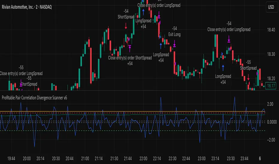
Profitable Pair Correlation Divergence Scanner v6This strategy identifies divergence opportunities between two correlated assets using a combination of Z-Score spread analysis, trend confirmation, RSI & MACD momentum checks, correlation filters, and ATR-based stop-loss/take-profit management. It’s optimized for positive P&L and realistic trade execution.
Key Features:
Pair Divergence Detection:
Measures deviation between returns of two assets and identifies overbought/oversold spread conditions using Z-Score.
Trend Alignment:
Trades only in the direction of the primary asset’s trend using a fast EMA vs slow EMA filter.
Momentum Confirmation:
Confirms trades with RSI and MACD to reduce false signals.
Correlation Filter:
Ensures the pair is strongly correlated before taking trades, avoiding noisy signals.
Risk Management:
Dynamic ATR-based stop-loss and take-profit ensures proper reward-to-risk ratio.
Exit Conditions:
Automatically closes positions when Z-Score normalizes, or ATR-based exits are hit.
How It Works:
Calculate Returns:
Computes returns for both assets over the selected timeframe.
Z-Score Spread:
Calculates the spread between returns and normalizes it using moving average and standard deviation.
Trend Filter:
Only takes long trades if the fast EMA is above the slow EMA, and short trades if the fast EMA is below the slow EMA.
Momentum Confirmation:
Confirms trade direction with RSI (>50 for longs, <50 for shorts) and MACD alignment.
Correlation Check:
Ensures the pair’s recent correlation is strong enough to validate divergence signals.
Trade Execution:
Opens positions when Z-Score crosses thresholds and all conditions align. Positions close when Z-Score normalizes or ATR-based SL/TP is hit.
Plot Explanation:
Z-Score: Blue line shows divergence magnitude.
Entry Levels: Red/Green lines mark long/short thresholds.
Exit Zone: Gray lines show normalization zone.
EMA Trend Lines: Purple (fast), Orange (slow) for trend alignment.
Correlation: Teal overlay shows current correlation strength.
Usage Tips:
Use highly correlated pairs for best results (e.g., EURUSD/GBPUSD).
Run on higher timeframe charts (1h or 4h) to reduce noise.
Adjust ATR multiplier based on volatility to avoid premature stops.
Combine with alerts for automated notifications or webhook execution.
Conclusion:
The Profitable Pair Correlation Divergence Scanner v6 is designed for traders who want systematic, low-risk, positive P&L trading opportunities with minimal manual monitoring. By combining trend alignment, momentum confirmation, correlation filters, and dynamic exits, it reduces false signals and improves execution reliability.
Run it on TradingView and watch how it captures divergence opportunities while maintaining positive P&L across trades.
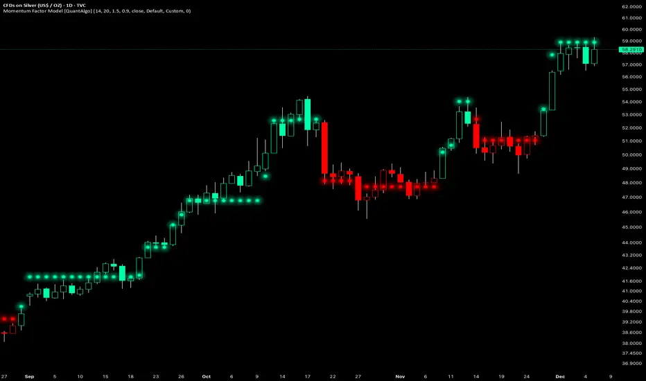
Momentum Factor Model [QuantAlgo]🟢 Overview
The Momentum Factor Model is a multi-horizon momentum analysis system that combines weighted return calculations with risk-adjusted price projections to identify and track persistent directional trends. The indicator employs a quantitative approach by measuring momentum across multiple timeframes simultaneously, applying exponential decay weighting to balance recent versus historical price action, and constructing volatility-normalized boundaries for trend validation. This factor-based methodology provides traders and investors with a systematic framework for momentum regime identification, trend persistence evaluation, and dynamic support/resistance determination across diverse market conditions and timeframes.
🟢 How It Works
The indicator constructs a composite momentum factor by calculating percentage returns over three distinct lookback periods (1, 3, and 5 bars) and combining them using exponentially decayed weights. The momentum decay parameter controls the relative importance of each timeframe, with higher decay values creating more balanced weighting between recent and historical momentum, while lower values emphasize immediate price action. This weighted momentum factor captures the multi-dimensional nature of trend strength rather than relying on a single timeframe measurement.
The expected return is derived by smoothing the momentum factor over a user-defined period, establishing a baseline for anticipated price movement based on recent momentum characteristics. This expected return then projects a factor-based price estimate, which undergoes risk adjustment through volatility normalization, creating a price estimate that accounts for both directional bias and market volatility conditions.
🟢 How to Use It
▶ Enter Long positions when the momentum factor dots (⏺) transition from red to green (bullish) , indicating the momentum factor model has confirmed positive directional bias. The color change represents a validated shift where the factor line has broken through the lower boundary and begun tracking the upper bound, signaling momentum reversal to the upside. Conversely, enter Short positions or exit existing Longs when the dots shift from green to red (bearish) , confirming negative momentum establishment and downward trend tracking.
The momentum factor dots function as a dynamic momentum-based reference pathway that can be used for position management and risk control. During bullish phases, the dot formation represents a momentum-weighted support zone where pullbacks may find stability before continuation. During bearish trends, it acts as resistance where rallies may encounter selling pressure. Price action relative to the momentum factor pathway provides context on trend health: sustained price movement in the direction of the trend (above the dots during bullish phases, below during bearish phases) confirms momentum persistence, while repeated violations may suggest weakening directional conviction.
▶ Configure alert notifications to monitor trend changes without continuous chart observation. The indicator provides three alert types: "Bullish Momentum Signal" triggers specifically on upward trend reversals, "Bearish Momentum Signal" captures downward momentum shifts, and "Momentum Trend Change" fires on any directional transition. These alerts activate only when the trend state changes from one regime to another, eliminating false triggers from intrabar noise or temporary boundary touches that don't result in confirmed trend reversals.
▶ The indicator also offers six pre-designed color schemes (Classic, Aqua, Cosmic, Ember, Neon, Custom) optimized for various chart backgrounds and visual preferences, ensuring the momentum trend remains clearly visible under different display conditions. The bar coloring feature overlays trend direction directly onto the price candles, providing immediate visual confirmation of the momentum regime without needing to reference the dot pattern position.
🟢 Pro Tips for Trading and Investing
▶ Align the configuration preset with your trading timeframe and objectives: Fast Response settings excel on 1-15 minute charts for scalping and day trading where capturing quick momentum shifts is paramount, though this comes with increased signal frequency and potential whipsaws in ranging conditions. Default parameters suit hourly to daily charts for swing trading, providing balanced responsiveness without excessive noise. Smooth Trend configuration works best on 4-hour to weekly timeframes for position trading and investment analysis, prioritizing trend stability over timing precision and significantly reducing false reversals during consolidation periods.
▶ Context matters significantly for momentum-based systems. The indicator performs optimally during trending market regimes where directional persistence exists and may struggle during sideways consolidation where momentum lacks consistency. Before taking signals, assess the broader market structure: look for established higher highs/higher lows (uptrend) or lower highs/lower lows (downtrend) on higher timeframes to confirm you're trading with the dominant directional bias. During range-bound periods, reduce position sizing or wait for the momentum factor dots to establish a clear directional slope and consistent movement before committing capital.
▶ Layer the momentum factor model with complementary analysis rather than using it in isolation. Combine trend signals with volume confirmation (increasing volume on trend changes suggests institutional participation), key support/resistance levels (signals near major levels carry higher probability), and volatility context (ATR expansion can precede significant moves). Consider the momentum decay parameter's impact: values near 0.85 make the model highly sensitive to recent price action, ideal for fast-moving markets but prone to false signals; values near 0.95 create smoother momentum estimates that better filter noise but may lag major reversals.
▶ Implement dynamic position management using the momentum factor pathway as a trailing reference framework. Rather than placing fixed stops, observe the dot formation's progression: as long as it maintains its directional slope and price respects it as support (bullish) or resistance (bearish), the momentum regime remains intact. Exit or tighten stops when price closes decisively through the momentum factor dots against your position, or when the dot pathway itself flattens (losing slope) indicating momentum exhaustion. For portfolio allocation, scale position sizes based on momentum factor strength, e.g., steeper dot progression angles and faster advancement suggest stronger momentum worthy of larger allocations within your risk parameters.
Session Opening Range Breakout (ORBO)This strategy automates a classic Opening Range Breakout (ORBO) approach: it builds a price range for the first minutes after the market opens, then looks for strong breakouts above or below that range to catch early directional moves.
Concept
The idea behind ORBO is simple:
The first minutes after the session open are often highly informative.
Price forms an “opening range” that acts as a mini support/resistance zone.
A clean breakout beyond this zone can lead to high-momentum moves.
This script turns that logic into a fully backtestable strategy in TradingView.
How the strategy works
Opening Range Session
Default session: 09:30–09:50 (exchange time)
During this window, the script tracks:
orHigh → highest high within the session
orLow → lowest low within the session
This forms your Opening Range for the day.
Breakout Logic (after the window ends)
Once the defined session ends:
Long Entry:
If the close crosses above the Opening Range High (orHigh),
→ strategy.entry("OR Long", strategy.long) is triggered.
Short Entry:
If the close crosses below the Opening Range Low (orLow),
→ strategy.entry("OR Short", strategy.short) is triggered.
Only one opening range per day is considered, which keeps the logic clean and easy to interpret.
Daily Reset
At the start of a new trading day, the script resets:
orHigh := na
orLow := na
A fresh Opening Range is then built using the next session’s 09:30–09:50 candles.
This ensures entries are always based on today’s structure, not yesterday’s.
Visuals & Inputs
Inputs:
Opening range session → default: "0930-0950"
Show OR levels → toggle visibility of OR High / Low lines
Fill range body → optional shaded zone between OR High and OR Low
Chart visuals:
A green line marks the Opening Range High.
A red line marks the Opening Range Low.
Optional yellow fill highlights the entire OR zone.
Background shading during the session shows when the range is currently being built.
These visuals make it easy to see:
Where the OR sits relative to current price
How clean / noisy the breakout was
How often price respects or rejects the opening zone
Backtesting & Optimization
Because this is written as a strategy():
You can use TradingView’s Strategy Tester to view:
Win rate
Net profit
Drawdown
Profit factor
Equity curve
Ideas to experiment with:
Change the session window (e.g., 09:15–09:45, 10:00–10:30)
Apply to different:
Markets: indices, FX, crypto, stocks
Timeframes: 1m / 5m / 15m
Add your own:
Stop Loss & Take Profit levels
Time filters (only trade certain days / times)
Volatility filters (e.g., ATR, range size thresholds)
Higher-timeframe trend filter (e.g., only take longs above 200 EMA)

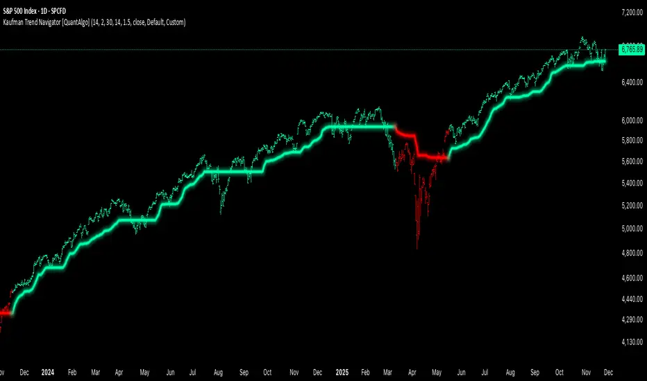
Kaufman Trend Navigator [QuantAlgo]🟢 Overview
The Kaufman Trend Navigator is an adaptive trend following system that combines efficiency-weighted price smoothing with volatility-adjusted bands to identify and track directional market movements. The indicator dynamically adjusts its sensitivity based on market conditions, becoming more responsive during trending periods and more conservative during consolidation. This dual-layer approach provides traders and investors with a systematic framework for trend identification, entry timing, and risk management across multiple timeframes and asset classes.
🟢 How It Works
The indicator employs an efficiency ratio mechanism that measures the directional movement of price relative to total price volatility over a defined lookback period. This ratio determines the adaptive response rate, allowing the system to distinguish between genuine directional moves and random market noise. When price exhibits strong directional characteristics, the internal smoothing accelerates to track the trend more closely. Conversely, during periods of low efficiency or choppy price action, the smoothing becomes more conservative to filter out false signals.
Volatility bands are constructed using normalized range measurements, creating dynamic upper and lower boundaries around the adaptive trend calculation. These bands expand and contract based on recent market volatility, providing context-dependent thresholds for trend validation. The trend line itself updates through a band-following logic where it tracks the relevant boundary based on the current directional bias, creating a stepping mechanism that maintains trend persistence while allowing for validated reversals.
The visual representation uses a gradient-weighted display to emphasize the primary trend line while maintaining clarity on price charts. Trend direction changes trigger when the internal logic confirms a boundary crossover, generating signals for potential position entries or exits. The system includes preset configurations calibrated for different trading timeframes, from responsive settings for scalping to smoother parameters suited for swing and position trading.
🟢 How to Use It
▶ Enter Long positions when the trend line transitions to Bullish (Green) coloring, which indicates upward directional bias has been established. Conversely, enter Short positions or exit Longs when the trend line shifts to Bearish (Red), which signals confirmed downward momentum.
The trend line itself can be used as dynamic support during uptrends and resistance during downtrends, providing logical areas for position management and stop placement. Price remaining above the line during bullish phases or below during bearish phases can also be used as a confirmation of trend strength and continuation probability.
▶ Built-in alert functionality provides real-time notifications for trend changes without requiring continuous chart monitoring. Configure alerts for Bullish Trend Signal to capture upward reversals, Bearish Trend Signal for downward shifts, or the general Trend Change alert to monitor both directions simultaneously. These alerts trigger only on confirmed trend transitions, reducing noise from intrabar fluctuations.
The indicator also includes six color presets (Classic, Aqua, Cosmic, Ember, Neon, Custom) to optimize visual clarity across different chart themes and lighting conditions. Select presets based on your monitor setup and background preference to ensure immediate trend recognition without visual strain. Bar coloring can be enabled to highlight trend direction directly on the price chart, eliminating the need to reference the trend line position during rapid market analysis.
🟢 Pro Tips for Trading and Investing
▶ Match the preset configuration (or your preferred settings) to your trading timeframe: use Fast Response for intraday charts (1-15 minutes), Default for swing trading (hourly to daily), and Smooth Trend for position trading (4-hour to weekly).
▶ Combine trend signals with volume analysis and market structure to filter lower-probability setups. During sideways markets, expect increased signal frequency with reduced reliability; consider waiting for the trend line to establish a clear slope before committing capital.
▶ Use the trend line as a trailing reference rather than a fixed stop level, allowing normal intrabar volatility while protecting against genuine reversals.
▶ For portfolio management, align position sizing with trend strength by observing the angle and consistency of the trend line progression.
Safe Supertrend Strategy (No Repaint)Overview
The Safe Supertrend is a repaint-free version of the popular Supertrend trend-following indicator.
Most Supertrend indicators appear perfect on historical charts because they flip intrabar and then repaint after the candle closes.
This version fixes that by using close-of-bar confirmation only, making every trend flip 100% stable, safe, and non-repainting.
Why This Supertrend Doesn’t Repaint
Most Supertrend indicators calculate their trend direction using the current bar’s data.
But during a live candle:
ATR expands and contracts
The upper/lower bands move
Price moves above/below the band temporarily
A false flip appears → then disappears when the candle closes
That is classic repainting.
This indicator avoids all of that by using:
close > upper
close < lower
This means:
Trend direction flips only based on the previous candle,
No intrabar calculations,
No flickering signals,
No “perfect but fake” historical performance.
Every signal you see on the chart is exactly what was available in real-time.
How It Works
Calculates ATR (Average True Range) and SMA centerline
Builds upper and lower volatility bands
Confirms trend flips only after the previous bar closes
Plots clear bull and bear reversal signals
Works on all markets (crypto, stocks, forex, indices)
No repainting, no recalc, no misleading flips.
Bullish Signal (Trend Up)
A bullish trend begins only when:
The previous candle closes above the upper ATR band,
And this flip is fully confirmed.
A green triangle marks the start of a new uptrend.
Bearish Signal (Trend Down)
A bearish trend begins only when:
The previous candle closes below the lower ATR band,
And the downtrend is confirmed.
A red triangle signals the start of a new downtrend.
Inputs
ATR Length - default 10
ATR Multiplier - default 3.0
Works on all timeframes and market
Simple, but powerful.
Why Use This Version Instead of a Regular Supertrend?
Most Supertrends:
Look great historically
But repaint continuously on live charts
Give false trend flips intrabar
Cannot be reliably used in strategies
This version:
Uses strict previous-bar logic
Never repaints trend direction
Works perfectly in live trading
Backtests accurately
Is ideal for algorithmic strategies
Ideal For:
Trend-following strategies
Breakout trading
Algo trading systems
Reversal detection
Filtering market noise
Swing trading & scalping
Final Note
This is a safer, more reliable Supertrend designed for real-world use — not perfect-looking repaint illusions.
If you use Supertrend in your trading system, this no-repaint version ensures your signals are trustworthy and consistent.

EMA Cross Strategy v5 (30 lots) (15 min candle only)- safe flip🚀 EMA Cross Strategy v5 (30 Lots) (15 min candle only)— Safe Flip Edition
Fully Automated | Fast | Reliable | Battle-tested
Welcome to a clean, powerful, and automation-friendly EMA crossover system.
This strategy is built for traders who want consistent trend-based entries without the risk of unwanted pyramiding or doubled positions.
🔥 How It Works
This strategy uses a fast EMA (10) crossing a slow EMA (20) to detect trend shifts:
Bullish Crossover → LONG (30 lots)
Bearish Crossover → SHORT (30 lots)
Every opposite signal safely flips the position by first closing the current trade, then opening a fresh position of exactly 30 lots.
No doubling.
No runaway position size.
No surprises.
Just clean, mechanical trend-following.
📈 Why This Strategy Stands Out
Unlike basic EMA crossbots, this version:
✔ Prevents unintended pyramiding
✔ Never over-allocates capital
✔ Works perfectly with webhook-based automation
✔ Produces stable, systematic entries
✔ Executes directional flips with precision
🔍 Backtest Highlights (1-Year)
(Backtests will vary by instrument/timeframe)
1,500+ trades executed
Profit factor above 1.27
Strong trend performance
Balanced long/short behavior
No margin calls
Consistent trade execution
This strategy thrives in trending markets and maintains strict discipline even in choppy conditions.
⚙️ Automation Ready
Designed for automated execution via webhook and API setups on supported platforms.
Just connect, run, and let the bot follow the rules without hesitation.
No emotions.
No overtrading.
No fear or greed.
Pure logic.

Frequency Momentum Oscillator [QuantAlgo]🟢 Overview
The Frequency Momentum Oscillator applies Fourier-based spectral analysis principles to price action to identify regime shifts and directional momentum. It calculates Fourier coefficients for selected harmonic frequencies on detrended price data, then measures the distribution of power across low, mid, and high frequency bands to distinguish between persistent directional trends and transient market noise. This approach provides traders with a quantitative framework for assessing whether current price action represents meaningful momentum or merely random fluctuations, enabling more informed entry and exit decisions across various asset classes and timeframes.
🟢 How It Works
The calculation process removes the dominant trend from price data by subtracting a simple moving average, isolating cyclical components for frequency analysis:
detrendedPrice = close - ta.sma(close , frequencyPeriod)
The detrended price series undergoes frequency decomposition through Fourier coefficient calculation across the first 8 harmonics. For each harmonic frequency, the algorithm computes sine and cosine components across the lookback window, then derives power as the sum of squared coefficients:
for k = 1 to 8
cosSum = 0.0
sinSum = 0.0
for n = 0 to frequencyPeriod - 1
angle = 2 * math.pi * k * n / frequencyPeriod
cosSum := cosSum + detrendedPrice * math.cos(angle)
sinSum := sinSum + detrendedPrice * math.sin(angle)
power = (cosSum * cosSum + sinSum * sinSum) / frequencyPeriod
Power measurements are aggregated into three frequency bands: low frequencies (harmonics 1-2) capturing persistent cycles, mid frequencies (harmonics 3-4), and high frequencies (harmonics 5-8) representing noise. Each band's power normalizes against total spectral power to create percentage distributions:
lowFreqNorm = totalPower > 0 ? (lowFreqPower / totalPower) * 100 : 33.33
highFreqNorm = totalPower > 0 ? (highFreqPower / totalPower) * 100 : 33.33
The normalized frequency components undergo exponential smoothing before calculating spectral balance as the difference between low and high frequency power:
smoothLow = ta.ema(lowFreqNorm, smoothingPeriod)
smoothHigh = ta.ema(highFreqNorm, smoothingPeriod)
spectralBalance = smoothLow - smoothHigh
Spectral balance combines with price momentum through directional multiplication, producing a composite signal that integrates frequency characteristics with price direction:
momentum = ta.change(close , frequencyPeriod/2)
compositeSignal = spectralBalance * math.sign(momentum)
finalSignal = ta.ema(compositeSignal, smoothingPeriod)
The final signal oscillates around zero, with positive values indicating low-frequency dominance coupled with upward momentum (trending up), and negative values indicating either high-frequency dominance (choppy market) or downward momentum (trending down).
🟢 How to Use This Indicator
→ Long/Short Signals: the indicator generates long signals when the smoothed composite signal crosses above zero (indicating low-frequency directional strength dominates) and short signals when it crosses below zero (indicating bearish momentum persistence).
→ Upper and Lower Reference Lines: the +25 and -25 reference lines serve as threshold markers for momentum strength. Readings beyond these levels indicate strong directional conviction, while oscillations between them suggest consolidation or weakening momentum. These references help traders distinguish between strong trending regimes and choppy transitional periods.
→ Preconfigured Presets: three optimized configurations are available with Default (32, 3) offering balanced responsiveness, Fast Response (24, 2) designed for scalping and intraday trading, and Smooth Trend (40, 5) calibrated for swing trading and position trading with enhanced noise filtration.
→ Built-in Alerts: the indicator includes three alert conditions for automated monitoring - Long Signal (momentum shifts bullish), Short Signal (momentum shifts bearish), and Signal Change (any directional transition). These alerts enable traders to receive real-time notifications without continuous chart monitoring.
→ Color Customization: four visual themes (Classic green/red, Aqua blue/orange, Cosmic aqua/purple, Custom) allow chart customization for different display environments and personal preferences.

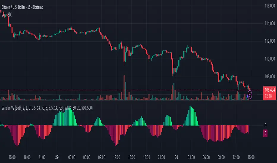
Vandan V2Vandan V2 is an automated trend-following strategy for NASDAQ E-mini Futures (NQ1!).
It uses multi-timeframe momentum and volatility filters to identify high-probability entries.
Includes dynamic risk management and trailing logic optimized for intraday trading.
Fisher Transform Trend Navigator [QuantAlgo]🟢 Overview
The Fisher Transform Trend Navigator applies a logarithmic transformation to normalize price data into a Gaussian distribution, then combines this with volatility-adaptive thresholds to create a trend detection system. This mathematical approach helps traders identify high-probability trend changes and reversal points while filtering market noise in the ever-changing volatility conditions.
🟢 How It Works
The indicator's foundation begins with price normalization, where recent price action is scaled to a bounded range between -1 and +1:
highestHigh = ta.highest(priceSource, fisherPeriod)
lowestLow = ta.lowest(priceSource, fisherPeriod)
value1 = highestHigh != lowestLow ? 2 * (priceSource - lowestLow) / (highestHigh - lowestLow) - 1 : 0
value1 := math.max(-0.999, math.min(0.999, value1))
This normalized value then passes through the Fisher Transform calculation, which applies a logarithmic function to convert the data into a Gaussian normal distribution that naturally amplifies price extremes and turning points:
fisherTransform = 0.5 * math.log((1 + value1) / (1 - value1))
smoothedFisher = ta.ema(fisherTransform, fisherSmoothing)
The smoothed Fisher signal is then integrated with an exponential moving average to create a hybrid trend line that balances statistical precision with price-following behavior:
baseTrend = ta.ema(close, basePeriod)
fisherAdjustment = smoothedFisher * fisherSensitivity * close
fisherTrend = baseTrend + fisherAdjustment
To filter out false signals and adapt to market conditions, the system calculates dynamic threshold bands using volatility measurements:
dynamicRange = ta.atr(volatilityPeriod)
threshold = dynamicRange * volatilityMultiplier
upperThreshold = fisherTrend + threshold
lowerThreshold = fisherTrend - threshold
When price momentum pushes through these thresholds, the trend line locks onto the new level and maintains direction until the opposite threshold is breached:
if upperThreshold < trendLine
trendLine := upperThreshold
if lowerThreshold > trendLine
trendLine := lowerThreshold
🟢 Signal Interpretation
Bullish Candles (Green): indicate normalized price distribution favoring bulls with sustained buying momentum = Long/Buy opportunities
Bearish Candles (Red): indicate normalized price distribution favoring bears with sustained selling pressure = Short/Sell opportunities
Upper Band Zone: Area above middle level indicating statistically elevated trend strength with potential overbought conditions approaching mean reversion zones
Lower Band Zone: Area below middle level indicating statistically depressed trend strength with potential oversold conditions approaching mean reversion zones
Built-in Alert System: Automated notifications trigger when bullish or bearish states change, allowing you to act on significant developments without constantly monitoring the charts
Candle Coloring: Optional feature applies trend colors to price bars for visual consistency and clarity
Configuration Presets: Three parameter sets available - Default (balanced settings), Scalping (faster response with higher sensitivity), and Swing Trading (slower response with enhanced smoothing)
Color Customization: Four color schemes including Classic, Aqua, Cosmic, and Custom options for personalized chart aesthetics

Bayesian Trend Navigator [QuantAlgo]🟢 Overview
The Bayesian Trend Navigator uses Bayesian statistics to continuously update trend probabilities by combining long-term expectations (prior beliefs) and short-term observations (likelihood evidence), rather than relying solely on recent price data like many conventional indicators. This mathematical framework produces robust directional signals that naturally balance responsiveness with stability, making it suitable for traders and investors seeking statistically-grounded trend identification across diverse market environments and asset types.
🟢 How It Works
The indicator operates on Bayesian inference principles, a statistical method for updating beliefs when new evidence emerges. The system begins by establishing a prior belief - a long-term trend expectation calculated from historical price behavior. This represents the "baseline hypothesis" about market direction before considering recent developments.
Simultaneously, the algorithm collects recent market evidence through short-term trend analysis, representing the likelihood component. This captures what current price action suggests about directional momentum independent of historical context.
The core Bayesian engine then combines these elements using conjugate normal distributions and precision weighting. It calculates prior precision (inverse variance) and likelihood precision, combining them to determine a posterior precision. The resulting posterior mean represents the mathematically optimal trend estimate given both historical patterns and current reality. This posterior calculation includes intervals derived from the posterior variance, providing probabilistic confidence bounds around the trend estimate.
Finally, volatility-based standard deviation bands create adaptive boundaries around the Bayesian estimate. The trend line adjusts within these constraints, generating color transitions between bullish (green) and bearish (red) states when the posterior calculation crosses these probabilistic thresholds.
🟢 How to Use
Green/Bullish Trend Line: Posterior probability favoring upward momentum, indicating statistically favorable conditions for long positions (buy)
Red/Bearish Trend Line: Posterior probability favoring downward momentum, signaling mathematically supported timing for short positions (sell)
Rising Green Line: Strengthening bullish posterior as new evidence reinforces upward beliefs, showing increasing probabilistic confidence in trend continuation with favorable long entry conditions
Declining Red Line: Intensifying bearish posterior with accumulating downside evidence, indicating growing statistical certainty in downtrend persistence and optimal short positioning opportunities
Flattening Trends: Diminishing posterior confidence regardless of color suggests equilibrium between prior beliefs and contradictory evidence, potentially signaling consolidation or insufficient statistical clarity for high-conviction trades
🟢 Pro Tips for Trading and Investing
→ Preset Configuration Strategy: Deploy presets based on your trading horizon - Scalping preset maximizes evidence weight (0.8) for rapid Bayesian updates on 1-15 minute charts, Default preset balances prior and likelihood for general applications, while Swing Trading preset equalizes weights (0.5/0.5) for stable inference on hourly and daily timeframes.
→ Prior Weight Adjustment: Calibrate prior weight according to market regime - increase values (0.5-0.7) in stable trending markets where historical patterns remain predictive, decrease values (0.2-0.3) during regime changes or news-driven volatility when recent evidence should dominate the posterior calculation.
→ Evidence Period Tuning: Modify the evidence period based on information flow velocity. Use shorter periods (5-8 bars) for assets with continuous price discovery like cryptocurrencies, medium periods (10-15) for liquid stocks, and longer periods (15-20) for slower-moving markets to ensure adequate likelihood sample size.
→ Likelihood Weight Optimization: Adjust likelihood weight inversely to market noise levels. Higher values (0.7-0.8) work well in clean trending conditions where recent data is reliable, while lower values (0.4-0.6) help during choppy periods by maintaining stronger reliance on established prior beliefs.
→ Multi-Timeframe Bayesian Confluence: Apply the indicator across multiple timeframes, using higher timeframes (Daily/Weekly) to establish prior belief direction and lower timeframes (Hourly/15-minute) for likelihood-driven entry timing, ensuring posterior probabilities align across temporal scales for maximum statistical confidence.
→ Standard Deviation Multiplier Management: Adapt the multiplier to match current uncertainty levels. Use tighter multipliers (1.0-1.5) during low-volatility consolidations to capture early trend emergence, and wider multipliers (2.0-2.5) during high-volatility events to avoid premature signals caused by statistical noise rather than genuine posterior shifts.
→ Variance-Based Position Sizing: Monitor the implicit posterior variance through trend line stability - smooth consistent movements indicate low uncertainty warranting larger positions, while erratic fluctuations suggest high statistical uncertainty calling for reduced exposure until clearer probabilistic convergence emerges.
→ Alert-Based Probabilistic Execution: Utilize trend change alerts to capture every statistically significant posterior shift from bullish to bearish states or vice versa without constantly monitoring the charts.

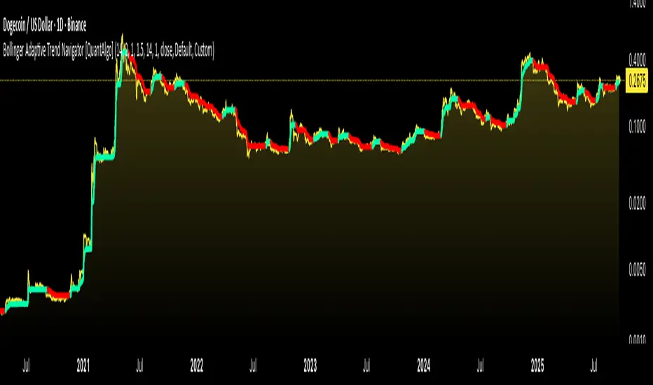
Bollinger Adaptive Trend Navigator [QuantAlgo]🟢 Overview
The Bollinger Adaptive Trend Navigator synthesizes volatility channel analysis with variable smoothing mechanics to generate trend identification signals. It uses price positioning within Bollinger Band structures to modify moving average responsiveness, while incorporating ATR calculations to establish trend line boundaries that constrain movement during volatile periods. The adaptive nature makes this indicator particularly valuable for traders and investors working across various asset classes including stocks, forex, commodities, and cryptocurrencies, with effectiveness spanning multiple timeframes from intraday scalping to longer-term position analysis.
🟢 How It Works
The core mechanism calculates price position within Bollinger Bands and uses this positioning to create an adaptive smoothing factor:
bbPosition = bbUpper != bbLower ? (source - bbLower) / (bbUpper - bbLower) : 0.5
adaptiveFactor = (bbPosition - 0.5) * 2 * adaptiveMultiplier * bandWidthRatio
alpha = math.max(0.01, math.min(0.5, 2.0 / (bbPeriod + 1) * (1 + math.abs(adaptiveFactor))))
This adaptive coefficient drives an exponential moving average that responds more aggressively when price approaches Bollinger Band extremes:
var float adaptiveTrend = source
adaptiveTrend := alpha * source + (1 - alpha) * nz(adaptiveTrend , source)
finalTrend = 0.7 * adaptiveTrend + 0.3 * smoothedCenter
ATR-based volatility boundaries constrain the final trend line to prevent excessive movement during volatile periods:
volatility = ta.atr(volatilityPeriod)
upperBound = bollingerTrendValue + (volatility * volatilityMultiplier)
lowerBound = bollingerTrendValue - (volatility * volatilityMultiplier)
The trend line direction determines bullish or bearish states through simple slope comparison, with the final output displaying color-coded signals based on the synthesis of Bollinger positioning, adaptive smoothing, and volatility constraints (green = long/buy, red = short/sell).
🟢 Signal Interpretation
Rising Trend Line (Green): Indicates upward direction based on Bollinger positioning and adaptive smoothing = Potential long/buy opportunity
Falling Trend Line (Red): Indicates downward direction based on Bollinger positioning and adaptive smoothing = Potential short/sell opportunity
Built-in Alert System: Automated notifications trigger when bullish or bearish states change, allowing you to act on significant development without constantly monitoring the charts
Candle Coloring: Optional feature applies trend colors to price bars for visual consistency
Configuration Presets: Three parameter sets available - Default (standard settings), Scalping (faster response), and Swing Trading (slower response)
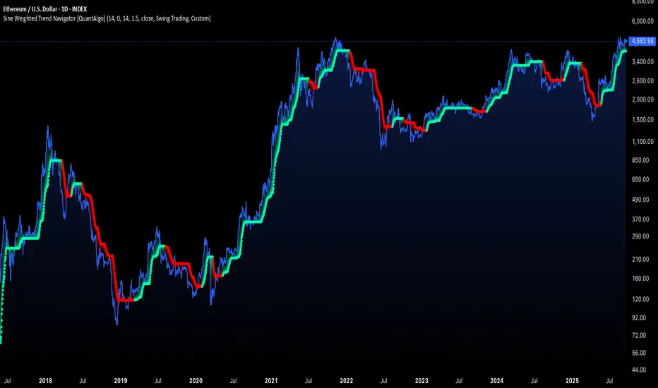
Sine Weighted Trend Navigator [QuantAlgo]🟢 Overview
The Sine Weighted Trend Navigator utilizes trigonometric mathematics to create a trend-following system that adapts to various market volatility. Unlike traditional moving averages that apply uniform weights, this indicator employs sine wave calculations to distribute weights across historical price data, creating a more responsive yet smooth trend measurement. Combined with volatility-adjusted boundaries, it produces actionable directional signals for traders and investors across various market conditions and asset classes.
🟢 How It Works
At its core, the indicator applies sine wave mathematics to weight historical prices. The system generates angular values across the lookback period and transforms them through sine calculations, creating a weight distribution pattern that naturally emphasizes recent price action while preserving smoothness. The phase shift feature allows rotation of this weighting pattern, enabling adjustment of the indicator's responsiveness to different market conditions.
Surrounding this sine-weighted calculation, the system establishes volatility-responsive boundaries through market volatility analysis. These boundaries expand and contract based on current market conditions, creating a dynamic framework that helps distinguish meaningful trend movements from random price fluctuations.
The trend determination logic compares the sine-weighted value against these adaptive boundaries. When the weighted value exceeds the upper boundary, it signals upward momentum. When it drops below the lower boundary, it indicates downward pressure. This comparison drives the color transitions of the main trend line, shifting between bullish (green) and bearish (red) states to provide clear directional guidance on price charts.
🟢 How to Use
Green/Bullish Trend Line: Rising momentum indicating optimal conditions for long positions (buy)
Red/Bearish Trend Line: Declining momentum signaling favorable timing for short positions (sell)
Steepening Green Line: Accelerating bullish momentum with increasing sine-weighted values indicating strengthening upward pressure and high-probability trend continuation
Steepening Red Line: Intensifying bearish momentum with declining sine-weighted calculations suggesting persistent downward pressure and optimal shorting opportunities
Flattening Trend Lines: Gradual reduction in directional momentum regardless of color may indicate approaching consolidation or trend exhaustion requiring position management review
🟢 Pro Tips for Trading and Investing
→ Preset Strategy Selection: Utilize the built-in presets strategically - Scalping preset for ultra-responsive 1-15 minute charts, Default preset for balanced general trading, and Swing Trading preset for 1-4 hour charts and multi-day positions.
→ Phase Shift Optimization: Fine-tune the phase shift parameter based on market bias - use positive values (0.1-0.5) in trending bull markets to enhance uptrend sensitivity, negative values (-0.1 to -0.5) in bear markets for improved downtrend detection, and zero for balanced neutral market conditions.
→ Multiplier Calibration: Adjust the multiplier according to market volatility and trading style. Use lower values (0.5-1.0) for tight, responsive signals in stable markets, higher values (2.0-3.0) during earnings seasons or high-volatility periods to filter noise and reduce whipsaws.
→ Sine Period Adaptation: Customize the sine weighted period based on your trading timeframe and market conditions. Use 5-14 for day trading to capture short-term momentum shifts, 14-25 for swing trading to balance responsiveness with reliability, and 25-50 for position trading to maintain long-term trend clarity.
→ Multi-Timeframe Sine Validation: Apply the indicator across multiple timeframes simultaneously, using higher timeframes (4H/Daily) for overall trend bias and lower timeframes (15m/1H) for entry timing, ensuring sine-weighted calculations align across different time horizons.
→ Alert-Driven Systematic Execution: Leverage the built-in trend change alerts to eliminate emotional decision-making and capture every mathematically-confirmed trend transition, particularly valuable for traders managing multiple instruments or those unable to monitor charts continuously.
→ Risk Management: Increase position sizes during strong directional sine-weighted momentum while reducing exposure during frequent color changes that indicate mathematical uncertainty or ranging market conditions lacking clear directional bias.
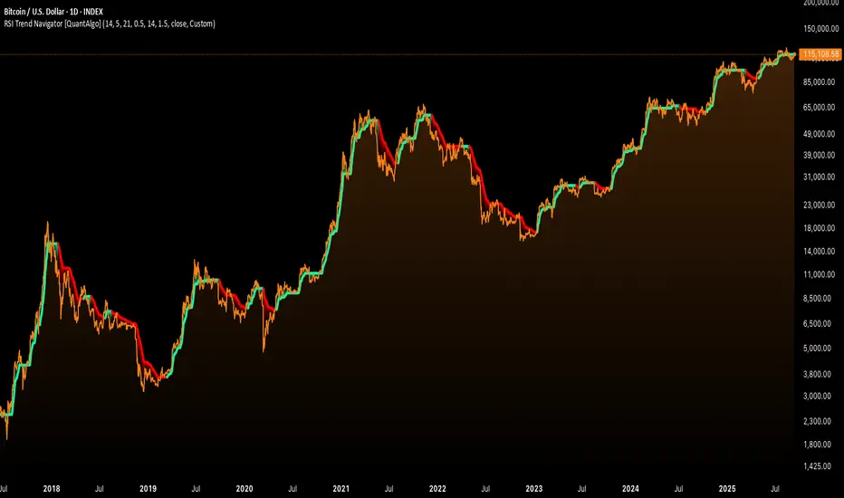
RSI Trend Navigator [QuantAlgo]🟢 Overview
The RSI Trend Navigator integrates RSI momentum calculations with adaptive exponential moving averages and ATR-based volatility bands to generate trend-following signals. The indicator applies variable smoothing coefficients based on RSI readings and incorporates normalized momentum adjustments to position a trend line that responds to both price action and underlying momentum conditions.
🟢 How It Works
The indicator begins by calculating and smoothing the RSI to reduce short-term fluctuations while preserving momentum information:
rsiValue = ta.rsi(source, rsiPeriod)
smoothedRSI = ta.ema(rsiValue, rsiSmoothing)
normalizedRSI = (smoothedRSI - 50) / 50
It then creates an adaptive smoothing coefficient that varies based on RSI positioning relative to the midpoint:
adaptiveAlpha = smoothedRSI > 50 ? 2.0 / (trendPeriod * 0.5 + 1) : 2.0 / (trendPeriod * 1.5 + 1)
This coefficient drives an adaptive trend calculation that responds more quickly when RSI indicates bullish momentum and more slowly during bearish conditions:
var float adaptiveTrend = source
adaptiveTrend := adaptiveAlpha * source + (1 - adaptiveAlpha) * nz(adaptiveTrend , source)
The normalized RSI values are converted into price-based adjustments using ATR for volatility scaling:
rsiAdjustment = normalizedRSI * ta.atr(14) * sensitivity
rsiTrendValue = adaptiveTrend + rsiAdjustment
ATR-based bands are constructed around this RSI-adjusted trend value to create dynamic boundaries that constrain trend line positioning:
atr = ta.atr(atrPeriod)
deviation = atr * atrMultiplier
upperBound = rsiTrendValue + deviation
lowerBound = rsiTrendValue - deviation
The trend line positioning uses these band constraints to determine its final value:
if upperBound < trendLine
trendLine := upperBound
if lowerBound > trendLine
trendLine := lowerBound
Signal generation occurs through directional comparison of the trend line against its previous value to establish bullish and bearish states:
trendUp = trendLine > trendLine
trendDown = trendLine < trendLine
if trendUp
isBullish := true
isBearish := false
else if trendDown
isBullish := false
isBearish := true
The final output colors the trend line green during bullish states and red during bearish states, creating visual buy/long and sell/short opportunity signals based on the combined RSI momentum and volatility-adjusted trend positioning.
🟢 Signal Interpretation
Rising Trend Line (Green): Indicates upward momentum where RSI influence and adaptive smoothing favor continued price advancement = Potential buy/long positions
Declining Trend Line (Red): Indicates downward momentum where RSI influence and adaptive smoothing favor continued price decline = Potential sell/short positions
Flattening Trend Lines: Occur when momentum weakens and the trend line slope approaches neutral, suggesting potential consolidation before the next move
Built-in Alert System: Automated notifications trigger when bullish or bearish states change, sending "RSI Trend Bullish Signal" or "RSI Trend Bearish Signal" messages for timely entry/exit
Color Bar Candles Option: Optional candle coloring feature that applies the same green/red trend colors to price bars, providing additional visual confirmation of the current trend direction

Sequential Pattern Strength [QuantAlgo]🟢 Overview
The Sequential Pattern Strength indicator measures the power and sustainability of consecutive price movements by tracking unbroken sequences of up or down closes. It incorporates sequence quality assessment, price extension analysis, and automatic exhaustion detection to help traders identify when strong trends are losing momentum and approaching potential reversal or continuation points.
🟢 How It Works
The indicator's key insight lies in its sequential pattern tracking system, where pattern strength is measured by analyzing consecutive price movements and their sustainability:
if close > close
upSequence := upSequence + 1
downSequence := 0
else if close < close
downSequence := downSequence + 1
upSequence := 0
The system calculates sequence quality by measuring how "perfect" the consecutive moves are:
perfectMoves = math.max(upSequence, downSequence)
totalMoves = math.abs(bar_index - ta.valuewhen(upSequence == 1 or downSequence == 1, bar_index, 0))
sequenceQuality = totalMoves > 0 ? perfectMoves / totalMoves : 1.0
First, it tracks price extension from the sequence starting point:
priceExtension = (close - sequenceStartPrice) / sequenceStartPrice * 100
Then, pattern exhaustion is identified when sequences become overextended:
isExhausted = math.abs(currentSequence) >= maxSequence or
math.abs(priceExtension) > resetThreshold * math.abs(currentSequence)
Finally, the pattern strength combines sequence length, quality, and price movement with momentum enhancement:
patternStrength = currentSequence * sequenceQuality * (1 + math.abs(priceExtension) / 10)
enhancedSignal = patternStrength + momentum * 10
signal = ta.ema(enhancedSignal, smooth)
This creates a sequence-based momentum indicator that combines consecutive movement analysis with pattern sustainability assessment, providing traders with both directional signals and exhaustion insights for entry/exit timing.
🟢 Signal Interpretation
Positive Values (Above Zero): Sequential pattern strength indicating bullish momentum with consecutive upward price movements and sustained buying pressure = Long/Buy opportunities
Negative Values (Below Zero): Sequential pattern strength indicating bearish momentum with consecutive downward price movements and sustained selling pressure = Short/Sell opportunities
Zero Line Crosses: Pattern transitions between bullish and bearish regimes, indicating potential trend changes or momentum shifts when sequences break
Upper Threshold Zone: Area above maximum sequence threshold (2x maxSequence) indicating extremely strong bullish patterns approaching exhaustion levels
Lower Threshold Zone: Area below negative threshold (-2x maxSequence) indicating extremely strong bearish patterns approaching exhaustion levels
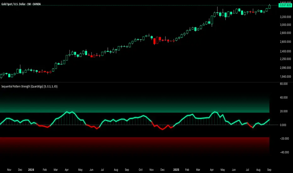
Divergence & Volume ThrustThis document provides both user and technical information for the "Divergence & Volume Thrust" (DVT) Pine Script indicator.
Part 1: User Guide
1.1 Introduction
The DVT indicator is an advanced tool designed to automatically identify high-probability trading setups. It works by detecting divergences between price and key momentum oscillators (RSI and MACD).
A divergence is a powerful signal that a trend might be losing strength and a reversal is possible. To filter out weak signals, the DVT indicator includes a Volume Thrust component, which ensures that a divergence is backed by significant market interest before it alerts you.
🐂 Bullish Divergence: Price makes a new low, but the indicator makes a higher low. This suggests selling pressure is weakening.
🐻 Bearish Divergence: Price makes a new high, but the indicator makes a lower high. This suggests buying pressure is weakening.
1.2 Key Features on Your Chart
When you add the indicator to your chart, here's what you will see:
Divergence Lines:
Bullish Lines (Teal): A line will be drawn on your chart connecting two price lows that form a bullish divergence.
Bearish Lines (Red): A line will be drawn connecting two price highs that form a bearish divergence.
Solid lines represent RSI divergences, while dashed lines represent MACD divergences.
Confirmation Labels:
"Bull Div ▲" (Teal Label): This label appears below the candle when a bullish divergence is detected and confirmed by a recent volume spike. This is a high-probability buy signal.
"Bear Div ▼" (Red Label): This label appears above the candle when a bearish divergence is detected and confirmed by a recent volume spike. This is a high-probability sell signal.
Volume Spike Bars (Orange Background):
Any price candle with a faint orange background indicates that the volume during that period was unusually high (exceeding the average volume by a multiplier you can set).
1.3 Settings and Configuration
You can customize the indicator to fit your trading style. Here's what each setting does:
Divergence Pivot Lookback (Left/Right): Controls the sensitivity of swing point detection. Lower numbers find smaller, more frequent divergences. Higher numbers find larger, more significant ones. 5 is a good starting point.
Max Lookback Range for Divergence: How many bars back the script will look for the first part of a divergence pattern. Default is 60.
Indicator Settings (RSI & MACD):
You can toggle RSI and MACD divergences on or off.
Standard length settings for each indicator (e.g., RSI Length 14, MACD 12, 26, 9).
Volume Settings:
Use Volume Confirmation: The most important filter. When checked, labels will only appear if a volume spike occurs near the divergence.
Volume MA Length: The lookback period for calculating average volume.
Volume Spike Multiplier: The core of the "Thrust" filter. A value of 2.0 means volume must be 200% (or 2x) the average to be considered a spike.
Visuals: Customize colors and toggle the confirmation labels on or off.
1.4 Strategy & Best Practices
Confluence is Key: The DVT indicator is powerful, but it should not be used in isolation. Look for its signals at key support and resistance levels, trendlines, or major moving averages for the highest probability setups.
Wait for Confirmation: A confirmed signal (with a label) is much more reliable than an unconfirmed divergence line.
Context Matters: A bullish divergence in a strong downtrend might only lead to a small bounce, not a full reversal. Use the signals in the context of the overall market structure.
Set Alerts: Use the TradingView alert system with this script. Create alerts for "Confirmed Bullish Divergence" and "Confirmed Bearish Divergence" to be notified of setups automatically.

Market Cap Landscape 3DHello, traders and creators! 👋
Market Cap Landscape 3D. This project is more than just a typical technical analysis tool; it's an exploration into what's possible when code meets artistry on the financial charts. It's a demonstration of how we can transcend flat, two-dimensional lines and step into a vibrant, three-dimensional world of data.
This project continues a journey that began with a previous 3D experiment, the T-Virus Sentiment, which you can explore here:
The Market Cap Landscape 3D builds on that foundation, visualizing market data—particularly crypto market caps—as a dynamic 3D mountain range. The entire landscape is procedurally generated and rendered in real-time using the powerful drawing capabilities of polyline.new() and line.new() , pushed to their creative limits.
This work is intended as a guide and a design example for all developers, born from the spirit of learning and a deep love for understanding the Pine Script™ language.
---
🧐 Core Concept: How It Works
The indicator synthesizes multiple layers of information into a single, cohesive 3D scene:
The Surface: The mountain range itself is a procedurally generated 3D mesh. Its peaks and valleys create a rich, textured landscape that serves as the canvas for our data.
Crypto Data Integration: The core feature is its ability to fetch market cap data for a list of cryptocurrencies you provide. It then sorts them in descending order and strategically places them onto the 3D surface.
The Summit: The highest point on the mountain is reserved for the asset with the #1 market cap in your list, visually represented by a flag and a custom emblem.
The Mountain Labels: The other assets are distributed across the mountainside, with their rank determining their general elevation. This creates an intuitive visual hierarchy.
The Leaderboard Pole: For clarity, a dedicated pole in the back-right corner provides a clean, ranked list of the symbols and their market caps, ensuring the data is always easy to read.
---
🧐 Example of adjusting the view
To evoke the feeling of flying over mountains
To evoke the feeling of looking at a mountain peak on a low plain
🧐 Example of predefined colors
---
🚀 How to Use
Getting started with the Market Cap Landscape 3D:
Add to Chart: Apply the "Market Cap Landscape 3D" indicator to your active chart.
Open Settings: Double-click anywhere on the 3D landscape or click the "Settings" icon next to the indicator's name.
Customize Your Crypto List: The most important setting is in the Crypto Data tab. In the "Symbols" text area, enter a comma-separated list of the crypto tickers you want to visualize (e.g., BTC,ETH,SOL,XRP ). The indicator supports up to 40 unique symbols.
> Important Note: This indicator exclusively uses TradingView's `CRYPTOCAP` data source. To find valid symbols, use the main symbol search bar on your chart. Type `CRYPTOCAP:` (including the colon) and you will see a list of available options. For example, typing `CRYPTOCAP:BTC` will confirm that `BTC` is a valid ticker for the indicator's settings. Using symbols that do not exist in the `CRYPTOCAP` index will result in a script error. or, to display other symbols, simply type CRYPTOCAP: (including the colon) and you will see a list of available options.
Adjust Your View: Use the settings in the Camera & Projection tab to rotate ( Yaw ), tilt ( Pitch ), and scale the landscape until you find a view you love.
Explore & Customize: Play with the color palettes, flag design, and other settings to make the landscape truly your own!
---
⚙️ Settings & Customization
This indicator is highly customizable. Here’s a breakdown of what each setting does:
#### 🪙 Crypto Data
Symbols: Enter the crypto tickers you want to track, separated by commas. The script automatically handles duplicates and case-insensitivity.
Show Market Cap on Mountain: When checked, it displays the full market cap value next to the symbol on the mountain. When unchecked, it shows a cleaner look with just the symbol and a colored circle background.
#### 📷 Camera & Projection
Yaw (°): Rotates the camera view horizontally (side to side).
Pitch (°): Tilts the camera view vertically (up and down).
Scale X, Y, Z: Stretches or compresses the landscape in width, depth, and height, respectively. Fine-tune these to get the perfect perspective.
#### 🏞️ Grid / Surface
Grid X/Y resolution: Controls the detail level of the 3D mesh. Higher values create a smoother surface but may use more resources.
Fill surface strips: Toggles the beautiful color gradient on the surface.
Show wireframe lines: Toggles the visibility of the grid lines.
Show nodes (markers): Toggles the small dots at each grid intersection point.
#### 🏔️ Peaks / Mountains
Fill peaks volume: Draws vertical lines on high peaks, giving them a sense of volume.
Fill peaks surface: Draws a cross-hatch pattern on the surface of high peaks.
Peak height threshold: Defines the minimum height for a peak to receive the fill effect.
Peak fill color/density: Customizes the appearance of the fill lines.
#### 🚩 Flags (3D)
Show Flag on Summit: A master switch to show or hide the flag and emblem entirely.
Flag height, width, etc.: Provides full control over the dimensions and orientation of the flag on the highest peak.
#### 🎨 Color Palette
Base Gradient Palette: Choose from 13 stunning, pre-designed color themes for the landscape, from the classic SUNSET_WAVE to vibrant themes like NEON_DREAM and OCEANIC .
#### 🛡️ Emblem / Badge Controls
This section gives you granular control over every element of the custom emblem on the flag. Tweak rotation, offsets, and scale to design your unique logo.
---
👨💻 Developer's Corner: Modifying the Core Logic
If you're a developer and wish to customize the indicator's core data source, this section is for you. The script is designed to be modular, making it easy to change what data is being ranked and visualized.
The heart of the data retrieval and ranking logic is within the f_getSortedCryptoData() function. Here’s how you can modify it:
1. Changing the Data Source (from Market Cap to something else):
The current logic uses request.security("CRYPTOCAP:" + syms.get(i), ...) to fetch market capitalization data. To change this, you need to modify this line.
Example: Ranking by RSI (14) on the Daily timeframe.
First, you'll need a function to calculate RSI. Add this function to the script:
f_getRSI(symbol, timeframe, length) =>
request.security(symbol, timeframe, ta.rsi(close, length))
Then, inside f_getSortedCryptoData() , find the `for` loop that populates the `caps` array and replace the `request.security` call:
// OLD LINE:
// caps.set(i, request.security("CRYPTOCAP:" + syms.get(i), timeframe.period, close))
// NEW LINE for RSI:
// Note: You'll need to decide how to format the symbol name (e.g., "BINANCE:" + syms.get(i) + "USDT")
caps.set(i, f_getRSI("BINANCE:" + syms.get(i) + "USDT", "D", 14))
2. Changing the Data Formatting:
The ranking values are formatted for display using the f_fmtCap() function, which currently formats large numbers into "M" (millions), "B" (billions), etc.
If you change the data source to something like RSI, you'll want to change the formatting. You can modify f_fmtCap() or create a new formatting function.
Example: Formatting for RSI.
// Modify f_fmtCap or create f_fmtRSI
f_fmtRSI(float v) =>
str.tostring(v, "#.##") // Simply format to two decimal places
Remember to update the calls to this function in the main drawing loop where the labels are created (e.g., str.format("{0}: {1}", crypto.symbol, f_fmtCap(crypto.cap)) ).
By modifying these key functions ( f_getSortedCryptoData and f_fmtCap ), you can adapt the Market Cap Landscape 3D to visualize and rank almost any dataset you can imagine, from technical indicators to fundamental data.
---
We hope you enjoy using the Market Cap Landscape 3D as much as we enjoyed creating it. Happy charting! ✨

Price Acceleration Matrix [QuantAlgo]🟢 Overview
The Price Acceleration Matrix indicator is an advanced momentum analysis tool that measures the rate of change in price velocity across multiple timeframes simultaneously. It transforms raw price data into velocity measurements for each timeframe, then calculates the acceleration of these velocities to identify when momentum is building or deteriorating. By analyzing acceleration alignment across all three timeframes, the system can distinguish between strong directional moves (all timeframes accelerating in the same direction) and weak, choppy movements (mixed acceleration signals). This multi-timeframe acceleration matrix provides traders with early warning signals for momentum shifts, trend continuation and reversal opportunities across different timeframes and asset classes.
🟢 How It Works
The indicator employs a three-stage calculation process that transforms price data into actionable acceleration signals. First, it calculates velocity (rate of price change) for each of the three user-defined timeframes by measuring the percentage change in price over the specified lookback periods. These velocity calculations are normalized by their respective timeframe lengths to ensure fair comparison across different periods.
In the second stage, the system calculates acceleration by measuring the change in velocity from one bar to the next for each timeframe, effectively capturing the second derivative of price movement. This acceleration data reveals whether momentum is building (positive acceleration) or deteriorating (negative acceleration) at each timeframe level.
The final stage creates the acceleration matrix score by evaluating alignment across all three timeframes. When all timeframes show positive acceleration, the system averages them for maximum bullish signal strength. When all show negative acceleration, it averages them for maximum bearish signal strength. However, when acceleration signals are mixed across timeframes, the system applies a penalty by dividing the average by two, indicating consolidation or conflicting momentum forces. The resulting signal is then smoothed using an Exponential Moving Average and scaled to the -3 to +3 range using a user-defined threshold parameter.
🟢 How to Use
1. Signal Interpretation and Momentum Analysis
Positive Territory (Above Zero): Indicates accelerating upward momentum with bullish bias and favorable conditions for long positions
Negative Territory (Below Zero): Signals accelerating downward momentum with bearish bias and favorable conditions for short positions
Extreme Levels (±2 to ±3): Represent maximum acceleration alignment across all timeframes, indicating high-probability momentum continuation
Moderate Levels (±1 to ±2): Suggest building momentum with good timeframe alignment but less conviction than extreme readings
Near Zero (-0.5 to +0.5): Indicates mixed signals, consolidation, or momentum exhaustion requiring caution
2. Overbought/Oversold Zone Analysis
Above +2 (Overbought Zone): Markets showing extreme bullish acceleration may be due for profit-taking or short-term pullbacks
Below -2 (Oversold Zone): Markets showing extreme bearish acceleration may present reversal opportunities or bounce potential
Zone Exits: When acceleration retreats from extreme zones, it often signals momentum exhaustion and potential trend changes
🟢 Pro Tips for Trading
→ Early Momentum Detection: Watch for acceleration crossing above zero after periods of negative readings, as this often precedes major price movements by several bars, providing early entry opportunities before traditional indicators signal.
→ Momentum Exhaustion Signals: Exit or take profits when acceleration reaches extreme levels (±2.5 or higher) and begins to decline, even if price continues in the same direction, as momentum deterioration typically precedes price reversals.
→ Acceleration Divergence Strategy: Look for divergences between price highs/lows and acceleration peaks/troughs, as these often signal weakening momentum and potential reversal opportunities before they become apparent on price charts.
→ Threshold Optimization: Adjust the acceleration threshold based on asset volatility - higher thresholds (0.7-1.0) for volatile assets to reduce false signals, lower thresholds (0.3-0.5) for stable assets to maintain sensitivity.
→ Alert-Based Trading: Utilize the built-in alert system for bullish/bearish reversals (±2 level crosses) and trend changes (zero line crosses) to capture momentum shifts without constant chart monitoring, especially effective for swing trading approaches.
→ Risk Management Integration: Reduce position sizes when acceleration readings are weak (below ±1.0) and increase allocation when strong acceleration alignment occurs (above ±2.0), as signal strength correlates directly with probability of successful trades.
