GKD-C STD-Filtered, Truncated Taylor FIR Filter [Loxx]Giga Kaleidoscope GKD-C STD-Filtered, Truncated Taylor Family FIR Filter is a Confirmation module included in Loxx's "Giga Kaleidoscope Modularized Trading System".
█ GKD-C STD-Filtered, Truncated Taylor Family FIR Filter
Exploring the Truncated Taylor Family FIR Filter with Standard Deviation Filtering
Filters play a vital role in signal processing, allowing us to extract valuable information from raw data by removing unwanted noise or highlighting specific features. In the context of financial data analysis, filtering techniques can help traders identify trends and make informed decisions. Below, we delve into the workings of a Truncated Taylor Family Finite Impulse Response (FIR) Filter with standard deviation filtering applied to the input and output signals. We will examine the code provided, breaking down the mathematical formulas and concepts behind it.
The code consists of two main sections: the design function that calculates the FIR filter coefficients and the stdFilter function that applies standard deviation filtering to the input signal.
design(int per, float taylorK)=>
float coeffs = array.new(per, 0)
float coeffsSum = 0
float _div = per + 1.0
float _coeff = 1
for i = 0 to per - 1
_coeff := (1 + taylorK) / 2 - (1 - taylorK) / 2 * math.cos(2.0 * math.pi * (i + 1) / _div)
array.set(coeffs,i, _coeff)
coeffsSum += _coeff
stdFilter(float src, int len, float filter)=>
float price = src
float filtdev = filter * ta.stdev(src, len)
price := math.abs(price - nz(price )) < filtdev ? nz(price ) : price
price
Design Function
The design function takes two arguments: an integer 'per' representing the number of coefficients for the FIR filter, and a floating-point number 'taylorK' to adjust the filter's characteristics. The function initializes an array 'coeffs' of length 'per' and sets all elements to 0. It also initializes variables 'coeffsSum', '_div', and '_coeff' to store the sum of the coefficients, a divisor for the cosine calculation, and the current coefficient, respectively.
A for loop iterates through the range of 0 to per-1, calculating the FIR filter coefficients using the formula:
_coeff := (1 + taylorK) / 2 - (1 - taylorK) / 2 * math.cos(2.0 * math.pi * (i + 1) / _div)
The calculated coefficients are stored in the 'coeffs' array, and their sum is stored in 'coeffsSum'. The function returns both 'coeffs' and 'coeffsSum' as a list.
stdFilter Function
The stdFilter function takes three arguments: a floating-point number 'src' representing the input signal, an integer 'len' for the standard deviation calculation period, and a floating-point number 'filter' to adjust the standard deviation filtering strength.
The function initializes a 'price' variable equal to 'src' and calculates the filtered standard deviation 'filtdev' using the formula:
filtdev = filter * ta.stdev(src, len)
The 'price' variable is then updated based on whether the absolute difference between the current price and the previous price is less than 'filtdev'. If true, 'price' is set to the previous price, effectively filtering out noise. Otherwise, 'price' remains unchanged.
Application of Design and stdFilter Functions
First, the input signal 'src' is filtered using the stdFilter function if the 'filterop' variable is set to "Both" or "Price", and 'filter' is greater than 0.
Next, the design function is called with the 'per' and 'taylorK' arguments to calculate the FIR filter coefficients and their sum. These values are stored in 'coeffs' and 'coeffsSum', respectively.
A for loop iterates through the range of 0 to per-1, calculating the filtered output 'dSum' using the formula:
dSum += nz(src ) * array.get(coeffs, k)
The output signal 'out' is then computed by dividing 'dSum' by 'coeffsSum' if 'coeffsSum' is not equal to 0; otherwise, 'out' is set to 0.
Finally, the output signal 'out' is filtered using the stdFilter function if the 'filterop' variable is set to "Both" or "Truncated Taylor FIR Filter", and 'filter' is greater than 0. The filtered signal is stored in the 'sig' variable.
The Truncated Taylor Family FIR Filter with Standard Deviation Filtering combines the strengths of two powerful filtering techniques to process financial data. By first designing the filter coefficients using the Taylor family FIR filter and then applying standard deviation filtering, the algorithm effectively removes noise and highlights relevant trends in the input signal. This approach allows traders and analysts to make more informed decisions based on the processed data.
In summary, the provided code effectively demonstrates how to create a custom FIR filter based on the Truncated Taylor family, along with standard deviation filtering applied to both input and output signals. This combination of filtering techniques enhances the overall filtering performance, making it a valuable tool for financial data analysis and decision-making processes. As the world of finance continues to evolve and generate increasingly complex data, the importance of robust and efficient filtering techniques cannot be overstated.
█ Giga Kaleidoscope Modularized Trading System
Core components of an NNFX algorithmic trading strategy
The NNFX algorithm is built on the principles of trend, momentum, and volatility. There are six core components in the NNFX trading algorithm:
1. Volatility - price volatility; e.g., Average True Range, True Range Double, Close-to-Close, etc.
2. Baseline - a moving average to identify price trend
3. Confirmation 1 - a technical indicator used to identify trends
4. Confirmation 2 - a technical indicator used to identify trends
5. Continuation - a technical indicator used to identify trends
6. Volatility/Volume - a technical indicator used to identify volatility/volume breakouts/breakdown
7. Exit - a technical indicator used to determine when a trend is exhausted
What is Volatility in the NNFX trading system?
In the NNFX (No Nonsense Forex) trading system, ATR (Average True Range) is typically used to measure the volatility of an asset. It is used as a part of the system to help determine the appropriate stop loss and take profit levels for a trade. ATR is calculated by taking the average of the true range values over a specified period.
True range is calculated as the maximum of the following values:
-Current high minus the current low
-Absolute value of the current high minus the previous close
-Absolute value of the current low minus the previous close
ATR is a dynamic indicator that changes with changes in volatility. As volatility increases, the value of ATR increases, and as volatility decreases, the value of ATR decreases. By using ATR in NNFX system, traders can adjust their stop loss and take profit levels according to the volatility of the asset being traded. This helps to ensure that the trade is given enough room to move, while also minimizing potential losses.
Other types of volatility include True Range Double (TRD), Close-to-Close, and Garman-Klass
What is a Baseline indicator?
The baseline is essentially a moving average, and is used to determine the overall direction of the market.
The baseline in the NNFX system is used to filter out trades that are not in line with the long-term trend of the market. The baseline is plotted on the chart along with other indicators, such as the Moving Average (MA), the Relative Strength Index (RSI), and the Average True Range (ATR).
Trades are only taken when the price is in the same direction as the baseline. For example, if the baseline is sloping upwards, only long trades are taken, and if the baseline is sloping downwards, only short trades are taken. This approach helps to ensure that trades are in line with the overall trend of the market, and reduces the risk of entering trades that are likely to fail.
By using a baseline in the NNFX system, traders can have a clear reference point for determining the overall trend of the market, and can make more informed trading decisions. The baseline helps to filter out noise and false signals, and ensures that trades are taken in the direction of the long-term trend.
What is a Confirmation indicator?
Confirmation indicators are technical indicators that are used to confirm the signals generated by primary indicators. Primary indicators are the core indicators used in the NNFX system, such as the Average True Range (ATR), the Moving Average (MA), and the Relative Strength Index (RSI).
The purpose of the confirmation indicators is to reduce false signals and improve the accuracy of the trading system. They are designed to confirm the signals generated by the primary indicators by providing additional information about the strength and direction of the trend.
Some examples of confirmation indicators that may be used in the NNFX system include the Bollinger Bands, the MACD (Moving Average Convergence Divergence), and the MACD Oscillator. These indicators can provide information about the volatility, momentum, and trend strength of the market, and can be used to confirm the signals generated by the primary indicators.
In the NNFX system, confirmation indicators are used in combination with primary indicators and other filters to create a trading system that is robust and reliable. By using multiple indicators to confirm trading signals, the system aims to reduce the risk of false signals and improve the overall profitability of the trades.
What is a Continuation indicator?
In the NNFX (No Nonsense Forex) trading system, a continuation indicator is a technical indicator that is used to confirm a current trend and predict that the trend is likely to continue in the same direction. A continuation indicator is typically used in conjunction with other indicators in the system, such as a baseline indicator, to provide a comprehensive trading strategy.
What is a Volatility/Volume indicator?
Volume indicators, such as the On Balance Volume (OBV), the Chaikin Money Flow (CMF), or the Volume Price Trend (VPT), are used to measure the amount of buying and selling activity in a market. They are based on the trading volume of the market, and can provide information about the strength of the trend. In the NNFX system, volume indicators are used to confirm trading signals generated by the Moving Average and the Relative Strength Index. Volatility indicators include Average Direction Index, Waddah Attar, and Volatility Ratio. In the NNFX trading system, volatility is a proxy for volume and vice versa.
By using volume indicators as confirmation tools, the NNFX trading system aims to reduce the risk of false signals and improve the overall profitability of trades. These indicators can provide additional information about the market that is not captured by the primary indicators, and can help traders to make more informed trading decisions. In addition, volume indicators can be used to identify potential changes in market trends and to confirm the strength of price movements.
What is an Exit indicator?
The exit indicator is used in conjunction with other indicators in the system, such as the Moving Average (MA), the Relative Strength Index (RSI), and the Average True Range (ATR), to provide a comprehensive trading strategy.
The exit indicator in the NNFX system can be any technical indicator that is deemed effective at identifying optimal exit points. Examples of exit indicators that are commonly used include the Parabolic SAR, the Average Directional Index (ADX), and the Chandelier Exit.
The purpose of the exit indicator is to identify when a trend is likely to reverse or when the market conditions have changed, signaling the need to exit a trade. By using an exit indicator, traders can manage their risk and prevent significant losses.
In the NNFX system, the exit indicator is used in conjunction with a stop loss and a take profit order to maximize profits and minimize losses. The stop loss order is used to limit the amount of loss that can be incurred if the trade goes against the trader, while the take profit order is used to lock in profits when the trade is moving in the trader's favor.
Overall, the use of an exit indicator in the NNFX trading system is an important component of a comprehensive trading strategy. It allows traders to manage their risk effectively and improve the profitability of their trades by exiting at the right time.
How does Loxx's GKD (Giga Kaleidoscope Modularized Trading System) implement the NNFX algorithm outlined above?
Loxx's GKD v1.0 system has five types of modules (indicators/strategies). These modules are:
1. GKD-BT - Backtesting module (Volatility, Number 1 in the NNFX algorithm)
2. GKD-B - Baseline module (Baseline and Volatility/Volume, Numbers 1 and 2 in the NNFX algorithm)
3. GKD-C - Confirmation 1/2 and Continuation module (Confirmation 1/2 and Continuation, Numbers 3, 4, and 5 in the NNFX algorithm)
4. GKD-V - Volatility/Volume module (Confirmation 1/2, Number 6 in the NNFX algorithm)
5. GKD-E - Exit module (Exit, Number 7 in the NNFX algorithm)
(additional module types will added in future releases)
Each module interacts with every module by passing data between modules. Data is passed between each module as described below:
GKD-B => GKD-V => GKD-C(1) => GKD-C(2) => GKD-C(Continuation) => GKD-E => GKD-BT
That is, the Baseline indicator passes its data to Volatility/Volume. The Volatility/Volume indicator passes its values to the Confirmation 1 indicator. The Confirmation 1 indicator passes its values to the Confirmation 2 indicator. The Confirmation 2 indicator passes its values to the Continuation indicator. The Continuation indicator passes its values to the Exit indicator, and finally, the Exit indicator passes its values to the Backtest strategy.
This chaining of indicators requires that each module conform to Loxx's GKD protocol, therefore allowing for the testing of every possible combination of technical indicators that make up the six components of the NNFX algorithm.
What does the application of the GKD trading system look like?
Example trading system:
Backtest: Strategy with 1-3 take profits, trailing stop loss, multiple types of PnL volatility, and 2 backtesting styles
Baseline: Hull Moving Average
Volatility/Volume: Hurst Exponent
Confirmation 1: STD-Filtered, Truncated Taylor Family FIR Filter as shown on the chart above
Confirmation 2: Williams Percent Range
Continuation: Fisher Transform
Exit: Rex Oscillator
Each GKD indicator is denoted with a module identifier of either: GKD-BT, GKD-B, GKD-C, GKD-V, or GKD-E. This allows traders to understand to which module each indicator belongs and where each indicator fits into the GKD protocol chain.
Giga Kaleidoscope Modularized Trading System Signals (based on the NNFX algorithm)
Standard Entry
1. GKD-C Confirmation 1 Signal
2. GKD-B Baseline agrees
3. Price is within a range of 0.2x Volatility and 1.0x Volatility of the Goldie Locks Mean
4. GKD-C Confirmation 2 agrees
5. GKD-V Volatility/Volume agrees
Baseline Entry
1. GKD-B Baseline signal
2. GKD-C Confirmation 1 agrees
3. Price is within a range of 0.2x Volatility and 1.0x Volatility of the Goldie Locks Mean
4. GKD-C Confirmation 2 agrees
5. GKD-V Volatility/Volume agrees
6. GKD-C Confirmation 1 signal was less than 7 candles prior
Volatility/Volume Entry
1. GKD-V Volatility/Volume signal
2. GKD-C Confirmation 1 agrees
3. Price is within a range of 0.2x Volatility and 1.0x Volatility of the Goldie Locks Mean
4. GKD-C Confirmation 2 agrees
5. GKD-B Baseline agrees
6. GKD-C Confirmation 1 signal was less than 7 candles prior
Continuation Entry
1. Standard Entry, Baseline Entry, or Pullback; entry triggered previously
2. GKD-B Baseline hasn't crossed since entry signal trigger
3. GKD-C Confirmation Continuation Indicator signals
4. GKD-C Confirmation 1 agrees
5. GKD-B Baseline agrees
6. GKD-C Confirmation 2 agrees
1-Candle Rule Standard Entry
1. GKD-C Confirmation 1 signal
2. GKD-B Baseline agrees
3. Price is within a range of 0.2x Volatility and 1.0x Volatility of the Goldie Locks Mean
Next Candle:
1. Price retraced (Long: close < close or Short: close > close )
2. GKD-B Baseline agrees
3. GKD-C Confirmation 1 agrees
4. GKD-C Confirmation 2 agrees
5. GKD-V Volatility/Volume agrees
1-Candle Rule Baseline Entry
1. GKD-B Baseline signal
2. GKD-C Confirmation 1 agrees
3. Price is within a range of 0.2x Volatility and 1.0x Volatility of the Goldie Locks Mean
4. GKD-C Confirmation 1 signal was less than 7 candles prior
Next Candle:
1. Price retraced (Long: close < close or Short: close > close )
2. GKD-B Baseline agrees
3. GKD-C Confirmation 1 agrees
4. GKD-C Confirmation 2 agrees
5. GKD-V Volatility/Volume Agrees
1-Candle Rule Volatility/Volume Entry
1. GKD-V Volatility/Volume signal
2. GKD-C Confirmation 1 agrees
3. Price is within a range of 0.2x Volatility and 1.0x Volatility of the Goldie Locks Mean
4. GKD-C Confirmation 1 signal was less than 7 candles prior
Next Candle:
1. Price retraced (Long: close < close or Short: close > close)
2. GKD-B Volatility/Volume agrees
3. GKD-C Confirmation 1 agrees
4. GKD-C Confirmation 2 agrees
5. GKD-B Baseline agrees
PullBack Entry
1. GKD-B Baseline signal
2. GKD-C Confirmation 1 agrees
3. Price is beyond 1.0x Volatility of Baseline
Next Candle:
1. Price is within a range of 0.2x Volatility and 1.0x Volatility of the Goldie Locks Mean
2. GKD-C Confirmation 1 agrees
3. GKD-C Confirmation 2 agrees
4. GKD-V Volatility/Volume Agrees
]█ Setting up the GKD
The GKD system involves chaining indicators together. These are the steps to set this up.
Use a GKD-C indicator alone on a chart
1. Inside the GKD-C indicator, change the "Confirmation Type" setting to "Solo Confirmation Simple"
Use a GKD-V indicator alone on a chart
**nothing, it's already useable on the chart without any settings changes
Use a GKD-B indicator alone on a chart
**nothing, it's already useable on the chart without any settings changes
Baseline (Baseline, Backtest)
1. Import the GKD-B Baseline into the GKD-BT Backtest: "Input into Volatility/Volume or Backtest (Baseline testing)"
2. Inside the GKD-BT Backtest, change the setting "Backtest Special" to "Baseline"
Volatility/Volume (Volatility/Volume, Backte st)
1. Inside the GKD-V indicator, change the "Testing Type" setting to "Solo"
2. Inside the GKD-V indicator, change the "Signal Type" setting to "Crossing" (neither traditional nor both can be backtested)
3. Import the GKD-V indicator into the GKD-BT Backtest: "Input into C1 or Backtest"
4. Inside the GKD-BT Backtest, change the setting "Backtest Special" to "Volatility/Volume"
5. Inside the GKD-BT Backtest, a) change the setting "Backtest Type" to "Trading" if using a directional GKD-V indicator; or, b) change the setting "Backtest Type" to "Full" if using a directional or non-directional GKD-V indicator (non-directional GKD-V can only test Longs and Shorts separately)
6. If "Backtest Type" is set to "Full": Inside the GKD-BT Backtest, change the setting "Backtest Side" to "Long" or "Short
7. If "Backtest Type" is set to "Full": To allow the system to open multiple orders at one time so you test all Longs or Shorts, open the GKD-BT Backtest, click the tab "Properties" and then insert a value of something like 10 orders into the "Pyramiding" settings. This will allow 10 orders to be opened at one time which should be enough to catch all possible Longs or Shorts.
Solo Confirmation Simple (Confirmation, Backtest)
1. Inside the GKD-C indicator, change the "Confirmation Type" setting to "Solo Confirmation Simple"
1. Import the GKD-C indicator into the GKD-BT Backtest: "Input into Backtest"
2. Inside the GKD-BT Backtest, change the setting "Backtest Special" to "Solo Confirmation Simple"
Solo Confirmation Complex without Exits (Baseline, Volatility/Volume, Confirmation, Backtest)
1. Inside the GKD-V indicator, change the "Testing Type" setting to "Chained"
2. Import the GKD-B Baseline into the GKD-V indicator: "Input into Volatility/Volume or Backtest (Baseline testing)"
3. Inside the GKD-C indicator, change the "Confirmation Type" setting to "Solo Confirmation Complex"
4. Import the GKD-V indicator into the GKD-C indicator: "Input into C1 or Backtest"
5. Inside the GKD-BT Backtest, change the setting "Backtest Special" to "GKD Full wo/ Exits"
6. Import the GKD-C into the GKD-BT Backtest: "Input into Exit or Backtest"
Solo Confirmation Complex with Exits (Baseline, Volatility/Volume, Confirmation, Exit, Backtest)
1. Inside the GKD-V indicator, change the "Testing Type" setting to "Chained"
2. Import the GKD-B Baseline into the GKD-V indicator: "Input into Volatility/Volume or Backtest (Baseline testing)"
3. Inside the GKD-C indicator, change the "Confirmation Type" setting to "Solo Confirmation Complex"
4. Import the GKD-V indicator into the GKD-C indicator: "Input into C1 or Backtest"
5. Import the GKD-C indicator into the GKD-E indicator: "Input into Exit"
6. Inside the GKD-BT Backtest, change the setting "Backtest Special" to "GKD Full w/ Exits"
7. Import the GKD-E into the GKD-BT Backtest: "Input into Backtest"
Full GKD without Exits (Baseline, Volatility/Volume, Confirmation 1, Confirmation 2, Continuation, Backtest)
1. Inside the GKD-V indicator, change the "Testing Type" setting to "Chained"
2. Import the GKD-B Baseline into the GKD-V indicator: "Input into Volatility/Volume or Backtest (Baseline testing)"
3. Inside the GKD-C 1 indicator, change the "Confirmation Type" setting to "Confirmation 1"
4. Import the GKD-V indicator into the GKD-C 1 indicator: "Input into C1 or Backtest"
5. Inside the GKD-C 2 indicator, change the "Confirmation Type" setting to "Confirmation 2"
6. Import the GKD-C 1 indicator into the GKD-C 2 indicator: "Input into C2"
7. Inside the GKD-C Continuation indicator, change the "Confirmation Type" setting to "Continuation"
8. Inside the GKD-BT Backtest, change the setting "Backtest Special" to "GKD Full wo/ Exits"
9. Import the GKD-E into the GKD-BT Backtest: "Input into Exit or Backtest"
Full GKD with Exits (Baseline, Volatility/Volume, Confirmation 1, Confirmation 2, Continuation, Exit, Backtest)
1. Inside the GKD-V indicator, change the "Testing Type" setting to "Chained"
2. Import the GKD-B Baseline into the GKD-V indicator: "Input into Volatility/Volume or Backtest (Baseline testing)"
3. Inside the GKD-C 1 indicator, change the "Confirmation Type" setting to "Confirmation 1"
4. Import the GKD-V indicator into the GKD-C 1 indicator: "Input into C1 or Backtest"
5. Inside the GKD-C 2 indicator, change the "Confirmation Type" setting to "Confirmation 2"
6. Import the GKD-C 1 indicator into the GKD-C 2 indicator: "Input into C2"
7. Inside the GKD-C Continuation indicator, change the "Confirmation Type" setting to "Continuation"
8. Import the GKD-C Continuation indicator into the GKD-E indicator: "Input into Exit"
9. Inside the GKD-BT Backtest, change the setting "Backtest Special" to "GKD Full w/ Exits"
10. Import the GKD-E into the GKD-BT Backtest: "Input into Backtest"
Baseline + Volatility/Volume (Baseline, Volatility/Volume, Backtest)
1. Inside the GKD-V indicator, change the "Testing Type" setting to "Baseline + Volatility/Volume"
2. Inside the GKD-V indicator, make sure the "Signal Type" setting is set to "Traditional"
3. Import the GKD-B Baseline into the GKD-V indicator: "Input into Volatility/Volume or Backtest (Baseline testing)"
4. Inside the GKD-BT Backtest, change the setting "Backtest Special" to "Baseline + Volatility/Volume"
5. Import the GKD-V into the GKD-BT Backtest: "Input into C1 or Backtest"
6. Inside the GKD-BT Backtest, change the setting "Backtest Type" to "Full". For this backtest, you must test Longs and Shorts separately
7. To allow the system to open multiple orders at one time so you can test all Longs or Shorts, open the GKD-BT Backtest, click the tab "Properties" and then insert a value of something like 10 orders into the "Pyramiding" settings. This will allow 10 orders to be opened at one time which should be enough to catch all possible Longs or Shorts.
Requirements
Inputs
Confirmation 1: GKD-V Volatility / Volume indicator
Confirmation 2: GKD-C Confirmation indicator
Continuation: GKD-C Confirmation indicator
Solo Confirmation Simple: GKD-B Baseline
Solo Confirmation Complex: GKD-V Volatility / Volume indicator
Solo Confirmation Super Complex: GKD-V Volatility / Volume indicator
Stacked 1: None
Stacked 2+: GKD-C, GKD-V, or GKD-B Stacked 1
Outputs
Confirmation 1: GKD-C Confirmation 2 indicator
Confirmation 2: GKD-C Continuation indicator
Continuation: GKD-E Exit indicator
Solo Confirmation Simple: GKD-BT Backtest
Solo Confirmation Complex: GKD-BT Backtest or GKD-E Exit indicator
Solo Confirmation Super Complex: GKD-C Continuation indicator
Stacked 1: GKD-C, GKD-V, or GKD-B Stacked 2+
Stacked 2+: GKD-C, GKD-V, or GKD-B Stacked 2+ or GKD-BT Backtest
Additional features will be added in future releases.
חפש סקריפטים עבור "algo"

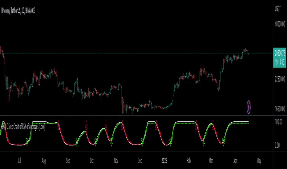
GKD-C Step Chart of RSX of Averages [Loxx]Giga Kaleidoscope GKD-C Step Chart of RSX of Averages is a Confirmation module included in Loxx's "Giga Kaleidoscope Modularized Trading System".
█ GKD-C Step Chart of RSX of Averages
What is the RSX?
The Jurik RSX is a technical indicator developed by Mark Jurik to measure the momentum and strength of price movements in financial markets, such as stocks, commodities, and currencies. It is an advanced version of the traditional Relative Strength Index (RSI), designed to offer smoother and less lagging signals compared to the standard RSI.
The main advantage of the Jurik RSX is that it provides more accurate and timely signals for traders and analysts, thanks to its improved calculation methods that reduce noise and lag in the indicator's output. This enables better decision-making when analyzing market trends and potential trading opportunities.
A Comprehensive Analysis of the stepChart() Algorithm for Financial Technical Analysis
Technical analysis is a widely adopted method for forecasting financial market trends by evaluating historical price data and utilizing various statistical tools. We examine an algorithm that implements the stepChart() function, a custom indicator designed to assist traders in identifying trends and making more informed decisions. We will provide an in-depth analysis of the code, exploring its structure, purpose, and functionality.
The code can be divided into two main sections: the stepChart() function definition and its application to charting data. We will first examine the stepChart() function definition, followed by its application.
stepChart() Function Definition
The stepChart() function takes two arguments: a floating-point number 'srcprice' representing the source price and a simple integer 'stepSize' to determine the increment for evaluating trends.
Within the function, five floating-point variables are initialized: steps, trend, rtrend, rbar_high, and rbar_low. These variables will be used to compute the step chart values and store the trends and bar high/low values.
The 'bar_index' variable is employed to identify the current bar in the price chart. If the current bar is the first one (bar_index == 0), the function initializes the steps, rbar_high, rbar_low, trend, and rtrend variables using the source price and step size. If stepSize is greater than 0, the variables are initialized using the rounded value of srcprice divided by stepSize, multiplied by stepSize. Otherwise, they are initialized to srcprice.
In the following part of the function, the code checks if the absolute difference between the source price and the previous steps value is less than the step size. If true, the current steps value remains unchanged. If not, the code enters a while loop that continues incrementing or decrementing the steps value by the step size until the absolute difference between the source price and the steps value is less than or equal to the step size.
Next, the trend variable is calculated based on the relationship between the current steps value and the previous steps value. The rbar_high, rbar_low, and rtrend variables are updated accordingly.
Finally, the function returns a list containing rbar_high, rbar_low, and rtrend values.
Application of the stepChart() Function
In this section, the stepChart() function is applied to the RSX of the smoothed moving average of the closing prices of a financial instrument. The moving average and RSX functions are used to calculate the moving average and RSX, respectively.
The stepChart() function is called with the RSX values and the user-defined step size. The resulting values are stored in the rbar_high, rbar_low, and rtrend variables.
Next, the bar_high, bar_low, bar_close, and bar_open variables are set based on the values of rbar_high, rbar_low, and rtrend. These variables will be used to plot the stepChart() on the price chart. The bar_high variable is set to rbar_high, and the bar_low variable is set to rbar_high if rbar_high is equal to rbar_low, or to rbar_low otherwise. The bar_close variable is set to bar_high if rtrend equals 1, and to bar_low otherwise. Lastly, the bar_open variable is set to bar_low if rtrend equals 1, and to bar_high otherwise.
Finally, we use the built in Pine function plotcandle to plot the candles on the chart.
The stepChart() function is an innovative technical analysis tool designed to help traders identify trends in financial markets. By combining the RSX and moving average indicators and utilizing the step chart approach, this custom indicator provides a visually appealing and intuitive representation of price trends. Understanding the intricacies of this code can prove invaluable for traders looking to make well-informed decisions
Core components of an NNFX algorithmic trading strategy
The NNFX algorithm is built on the principles of trend, momentum, and volatility. There are six core components in the NNFX trading algorithm:
1. Volatility - price volatility; e.g., Average True Range, True Range Double, Close-to-Close, etc.
2. Baseline - a moving average to identify price trend
3. Confirmation 1 - a technical indicator used to identify trends
4. Confirmation 2 - a technical indicator used to identify trends
5. Continuation - a technical indicator used to identify trends
6. Volatility/Volume - a technical indicator used to identify volatility/volume breakouts/breakdown
7. Exit - a technical indicator used to determine when a trend is exhausted
What is Volatility in the NNFX trading system?
In the NNFX (No Nonsense Forex) trading system, ATR (Average True Range) is typically used to measure the volatility of an asset. It is used as a part of the system to help determine the appropriate stop loss and take profit levels for a trade. ATR is calculated by taking the average of the true range values over a specified period.
True range is calculated as the maximum of the following values:
-Current high minus the current low
-Absolute value of the current high minus the previous close
-Absolute value of the current low minus the previous close
ATR is a dynamic indicator that changes with changes in volatility. As volatility increases, the value of ATR increases, and as volatility decreases, the value of ATR decreases. By using ATR in NNFX system, traders can adjust their stop loss and take profit levels according to the volatility of the asset being traded. This helps to ensure that the trade is given enough room to move, while also minimizing potential losses.
Other types of volatility include True Range Double (TRD), Close-to-Close, and Garman-Klass
What is a Baseline indicator?
The baseline is essentially a moving average, and is used to determine the overall direction of the market.
The baseline in the NNFX system is used to filter out trades that are not in line with the long-term trend of the market. The baseline is plotted on the chart along with other indicators, such as the Moving Average (MA), the Relative Strength Index (RSI), and the Average True Range (ATR).
Trades are only taken when the price is in the same direction as the baseline. For example, if the baseline is sloping upwards, only long trades are taken, and if the baseline is sloping downwards, only short trades are taken. This approach helps to ensure that trades are in line with the overall trend of the market, and reduces the risk of entering trades that are likely to fail.
By using a baseline in the NNFX system, traders can have a clear reference point for determining the overall trend of the market, and can make more informed trading decisions. The baseline helps to filter out noise and false signals, and ensures that trades are taken in the direction of the long-term trend.
What is a Confirmation indicator?
Confirmation indicators are technical indicators that are used to confirm the signals generated by primary indicators. Primary indicators are the core indicators used in the NNFX system, such as the Average True Range (ATR), the Moving Average (MA), and the Relative Strength Index (RSI).
The purpose of the confirmation indicators is to reduce false signals and improve the accuracy of the trading system. They are designed to confirm the signals generated by the primary indicators by providing additional information about the strength and direction of the trend.
Some examples of confirmation indicators that may be used in the NNFX system include the Bollinger Bands, the MACD (Moving Average Convergence Divergence), and the MACD Oscillator. These indicators can provide information about the volatility, momentum, and trend strength of the market, and can be used to confirm the signals generated by the primary indicators.
In the NNFX system, confirmation indicators are used in combination with primary indicators and other filters to create a trading system that is robust and reliable. By using multiple indicators to confirm trading signals, the system aims to reduce the risk of false signals and improve the overall profitability of the trades.
What is a Continuation indicator?
In the NNFX (No Nonsense Forex) trading system, a continuation indicator is a technical indicator that is used to confirm a current trend and predict that the trend is likely to continue in the same direction. A continuation indicator is typically used in conjunction with other indicators in the system, such as a baseline indicator, to provide a comprehensive trading strategy.
What is a Volatility/Volume indicator?
Volume indicators, such as the On Balance Volume (OBV), the Chaikin Money Flow (CMF), or the Volume Price Trend (VPT), are used to measure the amount of buying and selling activity in a market. They are based on the trading volume of the market, and can provide information about the strength of the trend. In the NNFX system, volume indicators are used to confirm trading signals generated by the Moving Average and the Relative Strength Index. Volatility indicators include Average Direction Index, Waddah Attar, and Volatility Ratio. In the NNFX trading system, volatility is a proxy for volume and vice versa.
By using volume indicators as confirmation tools, the NNFX trading system aims to reduce the risk of false signals and improve the overall profitability of trades. These indicators can provide additional information about the market that is not captured by the primary indicators, and can help traders to make more informed trading decisions. In addition, volume indicators can be used to identify potential changes in market trends and to confirm the strength of price movements.
What is an Exit indicator?
The exit indicator is used in conjunction with other indicators in the system, such as the Moving Average (MA), the Relative Strength Index (RSI), and the Average True Range (ATR), to provide a comprehensive trading strategy.
The exit indicator in the NNFX system can be any technical indicator that is deemed effective at identifying optimal exit points. Examples of exit indicators that are commonly used include the Parabolic SAR, the Average Directional Index (ADX), and the Chandelier Exit.
The purpose of the exit indicator is to identify when a trend is likely to reverse or when the market conditions have changed, signaling the need to exit a trade. By using an exit indicator, traders can manage their risk and prevent significant losses.
In the NNFX system, the exit indicator is used in conjunction with a stop loss and a take profit order to maximize profits and minimize losses. The stop loss order is used to limit the amount of loss that can be incurred if the trade goes against the trader, while the take profit order is used to lock in profits when the trade is moving in the trader's favor.
Overall, the use of an exit indicator in the NNFX trading system is an important component of a comprehensive trading strategy. It allows traders to manage their risk effectively and improve the profitability of their trades by exiting at the right time.
How does Loxx's GKD (Giga Kaleidoscope Modularized Trading System) implement the NNFX algorithm outlined above?
Loxx's GKD v1.0 system has five types of modules (indicators/strategies). These modules are:
1. GKD-BT - Backtesting module (Volatility, Number 1 in the NNFX algorithm)
2. GKD-B - Baseline module (Baseline and Volatility/Volume, Numbers 1 and 2 in the NNFX algorithm)
3. GKD-C - Confirmation 1/2 and Continuation module (Confirmation 1/2 and Continuation, Numbers 3, 4, and 5 in the NNFX algorithm)
4. GKD-V - Volatility/Volume module (Confirmation 1/2, Number 6 in the NNFX algorithm)
5. GKD-E - Exit module (Exit, Number 7 in the NNFX algorithm)
(additional module types will added in future releases)
Each module interacts with every module by passing data between modules. Data is passed between each module as described below:
GKD-B => GKD-V => GKD-C(1) => GKD-C(2) => GKD-C(Continuation) => GKD-E => GKD-BT
That is, the Baseline indicator passes its data to Volatility/Volume. The Volatility/Volume indicator passes its values to the Confirmation 1 indicator. The Confirmation 1 indicator passes its values to the Confirmation 2 indicator. The Confirmation 2 indicator passes its values to the Continuation indicator. The Continuation indicator passes its values to the Exit indicator, and finally, the Exit indicator passes its values to the Backtest strategy.
This chaining of indicators requires that each module conform to Loxx's GKD protocol, therefore allowing for the testing of every possible combination of technical indicators that make up the six components of the NNFX algorithm.
What does the application of the GKD trading system look like?
Example trading system:
Backtest: Strategy with 1-3 take profits, trailing stop loss, multiple types of PnL volatility, and 2 backtesting styles
Baseline: Hull Moving Average
Volatility/Volume: Hurst Exponent
Confirmation 1: Step Chart of RSX of Averages as shown on the chart above
Confirmation 2: Williams Percent Range
Continuation: Fisher Transform
Exit: Rex Oscillator
Each GKD indicator is denoted with a module identifier of either: GKD-BT, GKD-B, GKD-C, GKD-V, or GKD-E. This allows traders to understand to which module each indicator belongs and where each indicator fits into the GKD protocol chain.
Giga Kaleidoscope Modularized Trading System Signals (based on the NNFX algorithm)
Standard Entry
1. GKD-C Confirmation 1 Signal
2. GKD-B Baseline agrees
3. Price is within a range of 0.2x Volatility and 1.0x Volatility of the Goldie Locks Mean
4. GKD-C Confirmation 2 agrees
5. GKD-V Volatility/Volume agrees
Baseline Entry
1. GKD-B Baseline signal
2. GKD-C Confirmation 1 agrees
3. Price is within a range of 0.2x Volatility and 1.0x Volatility of the Goldie Locks Mean
4. GKD-C Confirmation 2 agrees
5. GKD-V Volatility/Volume agrees
6. GKD-C Confirmation 1 signal was less than 7 candles prior
Volatility/Volume Entry
1. GKD-V Volatility/Volume signal
2. GKD-C Confirmation 1 agrees
3. Price is within a range of 0.2x Volatility and 1.0x Volatility of the Goldie Locks Mean
4. GKD-C Confirmation 2 agrees
5. GKD-B Baseline agrees
6. GKD-C Confirmation 1 signal was less than 7 candles prior
Continuation Entry
1. Standard Entry, Baseline Entry, or Pullback; entry triggered previously
2. GKD-B Baseline hasn't crossed since entry signal trigger
3. GKD-C Confirmation Continuation Indicator signals
4. GKD-C Confirmation 1 agrees
5. GKD-B Baseline agrees
6. GKD-C Confirmation 2 agrees
1-Candle Rule Standard Entry
1. GKD-C Confirmation 1 signal
2. GKD-B Baseline agrees
3. Price is within a range of 0.2x Volatility and 1.0x Volatility of the Goldie Locks Mean
Next Candle:
1. Price retraced (Long: close < close or Short: close > close )
2. GKD-B Baseline agrees
3. GKD-C Confirmation 1 agrees
4. GKD-C Confirmation 2 agrees
5. GKD-V Volatility/Volume agrees
1-Candle Rule Baseline Entry
1. GKD-B Baseline signal
2. GKD-C Confirmation 1 agrees
3. Price is within a range of 0.2x Volatility and 1.0x Volatility of the Goldie Locks Mean
4. GKD-C Confirmation 1 signal was less than 7 candles prior
Next Candle:
1. Price retraced (Long: close < close or Short: close > close )
2. GKD-B Baseline agrees
3. GKD-C Confirmation 1 agrees
4. GKD-C Confirmation 2 agrees
5. GKD-V Volatility/Volume Agrees
1-Candle Rule Volatility/Volume Entry
1. GKD-V Volatility/Volume signal
2. GKD-C Confirmation 1 agrees
3. Price is within a range of 0.2x Volatility and 1.0x Volatility of the Goldie Locks Mean
4. GKD-C Confirmation 1 signal was less than 7 candles prior
Next Candle:
1. Price retraced (Long: close < close or Short: close > close)
2. GKD-B Volatility/Volume agrees
3. GKD-C Confirmation 1 agrees
4. GKD-C Confirmation 2 agrees
5. GKD-B Baseline agrees
PullBack Entry
1. GKD-B Baseline signal
2. GKD-C Confirmation 1 agrees
3. Price is beyond 1.0x Volatility of Baseline
Next Candle:
1. Price is within a range of 0.2x Volatility and 1.0x Volatility of the Goldie Locks Mean
2. GKD-C Confirmation 1 agrees
3. GKD-C Confirmation 2 agrees
4. GKD-V Volatility/Volume Agrees
]█ Setting up the GKD
The GKD system involves chaining indicators together. These are the steps to set this up.
Use a GKD-C indicator alone on a chart
1. Inside the GKD-C indicator, change the "Confirmation Type" setting to "Solo Confirmation Simple"
Use a GKD-V indicator alone on a chart
**nothing, it's already useable on the chart without any settings changes
Use a GKD-B indicator alone on a chart
**nothing, it's already useable on the chart without any settings changes
Baseline (Baseline, Backtest)
1. Import the GKD-B Baseline into the GKD-BT Backtest: "Input into Volatility/Volume or Backtest (Baseline testing)"
2. Inside the GKD-BT Backtest, change the setting "Backtest Special" to "Baseline"
Volatility/Volume (Volatility/Volume, Backte st)
1. Inside the GKD-V indicator, change the "Testing Type" setting to "Solo"
2. Inside the GKD-V indicator, change the "Signal Type" setting to "Crossing" (neither traditional nor both can be backtested)
3. Import the GKD-V indicator into the GKD-BT Backtest: "Input into C1 or Backtest"
4. Inside the GKD-BT Backtest, change the setting "Backtest Special" to "Volatility/Volume"
5. Inside the GKD-BT Backtest, a) change the setting "Backtest Type" to "Trading" if using a directional GKD-V indicator; or, b) change the setting "Backtest Type" to "Full" if using a directional or non-directional GKD-V indicator (non-directional GKD-V can only test Longs and Shorts separately)
6. If "Backtest Type" is set to "Full": Inside the GKD-BT Backtest, change the setting "Backtest Side" to "Long" or "Short
7. If "Backtest Type" is set to "Full": To allow the system to open multiple orders at one time so you test all Longs or Shorts, open the GKD-BT Backtest, click the tab "Properties" and then insert a value of something like 10 orders into the "Pyramiding" settings. This will allow 10 orders to be opened at one time which should be enough to catch all possible Longs or Shorts.
Solo Confirmation Simple (Confirmation, Backtest)
1. Inside the GKD-C indicator, change the "Confirmation Type" setting to "Solo Confirmation Simple"
1. Import the GKD-C indicator into the GKD-BT Backtest: "Input into Backtest"
2. Inside the GKD-BT Backtest, change the setting "Backtest Special" to "Solo Confirmation Simple"
Solo Confirmation Complex without Exits (Baseline, Volatility/Volume, Confirmation, Backtest)
1. Inside the GKD-V indicator, change the "Testing Type" setting to "Chained"
2. Import the GKD-B Baseline into the GKD-V indicator: "Input into Volatility/Volume or Backtest (Baseline testing)"
3. Inside the GKD-C indicator, change the "Confirmation Type" setting to "Solo Confirmation Complex"
4. Import the GKD-V indicator into the GKD-C indicator: "Input into C1 or Backtest"
5. Inside the GKD-BT Backtest, change the setting "Backtest Special" to "GKD Full wo/ Exits"
6. Import the GKD-C into the GKD-BT Backtest: "Input into Exit or Backtest"
Solo Confirmation Complex with Exits (Baseline, Volatility/Volume, Confirmation, Exit, Backtest)
1. Inside the GKD-V indicator, change the "Testing Type" setting to "Chained"
2. Import the GKD-B Baseline into the GKD-V indicator: "Input into Volatility/Volume or Backtest (Baseline testing)"
3. Inside the GKD-C indicator, change the "Confirmation Type" setting to "Solo Confirmation Complex"
4. Import the GKD-V indicator into the GKD-C indicator: "Input into C1 or Backtest"
5. Import the GKD-C indicator into the GKD-E indicator: "Input into Exit"
6. Inside the GKD-BT Backtest, change the setting "Backtest Special" to "GKD Full w/ Exits"
7. Import the GKD-E into the GKD-BT Backtest: "Input into Backtest"
Full GKD without Exits (Baseline, Volatility/Volume, Confirmation 1, Confirmation 2, Continuation, Backtest)
1. Inside the GKD-V indicator, change the "Testing Type" setting to "Chained"
2. Import the GKD-B Baseline into the GKD-V indicator: "Input into Volatility/Volume or Backtest (Baseline testing)"
3. Inside the GKD-C 1 indicator, change the "Confirmation Type" setting to "Confirmation 1"
4. Import the GKD-V indicator into the GKD-C 1 indicator: "Input into C1 or Backtest"
5. Inside the GKD-C 2 indicator, change the "Confirmation Type" setting to "Confirmation 2"
6. Import the GKD-C 1 indicator into the GKD-C 2 indicator: "Input into C2"
7. Inside the GKD-C Continuation indicator, change the "Confirmation Type" setting to "Continuation"
8. Inside the GKD-BT Backtest, change the setting "Backtest Special" to "GKD Full wo/ Exits"
9. Import the GKD-E into the GKD-BT Backtest: "Input into Exit or Backtest"
Full GKD with Exits (Baseline, Volatility/Volume, Confirmation 1, Confirmation 2, Continuation, Exit, Backtest)
1. Inside the GKD-V indicator, change the "Testing Type" setting to "Chained"
2. Import the GKD-B Baseline into the GKD-V indicator: "Input into Volatility/Volume or Backtest (Baseline testing)"
3. Inside the GKD-C 1 indicator, change the "Confirmation Type" setting to "Confirmation 1"
4. Import the GKD-V indicator into the GKD-C 1 indicator: "Input into C1 or Backtest"
5. Inside the GKD-C 2 indicator, change the "Confirmation Type" setting to "Confirmation 2"
6. Import the GKD-C 1 indicator into the GKD-C 2 indicator: "Input into C2"
7. Inside the GKD-C Continuation indicator, change the "Confirmation Type" setting to "Continuation"
8. Import the GKD-C Continuation indicator into the GKD-E indicator: "Input into Exit"
9. Inside the GKD-BT Backtest, change the setting "Backtest Special" to "GKD Full w/ Exits"
10. Import the GKD-E into the GKD-BT Backtest: "Input into Backtest"
Baseline + Volatility/Volume (Baseline, Volatility/Volume, Backtest)
1. Inside the GKD-V indicator, change the "Testing Type" setting to "Baseline + Volatility/Volume"
2. Inside the GKD-V indicator, make sure the "Signal Type" setting is set to "Traditional"
3. Import the GKD-B Baseline into the GKD-V indicator: "Input into Volatility/Volume or Backtest (Baseline testing)"
4. Inside the GKD-BT Backtest, change the setting "Backtest Special" to "Baseline + Volatility/Volume"
5. Import the GKD-V into the GKD-BT Backtest: "Input into C1 or Backtest"
6. Inside the GKD-BT Backtest, change the setting "Backtest Type" to "Full". For this backtest, you must test Longs and Shorts separately
7. To allow the system to open multiple orders at one time so you can test all Longs or Shorts, open the GKD-BT Backtest, click the tab "Properties" and then insert a value of something like 10 orders into the "Pyramiding" settings. This will allow 10 orders to be opened at one time which should be enough to catch all possible Longs or Shorts.
Requirements
Inputs
Confirmation 1: GKD-V Volatility / Volume indicator
Confirmation 2: GKD-C Confirmation indicator
Continuation: GKD-C Confirmation indicator
Solo Confirmation Simple: GKD-B Baseline
Solo Confirmation Complex: GKD-V Volatility / Volume indicator
Solo Confirmation Super Complex: GKD-V Volatility / Volume indicator
Stacked 1: None
Stacked 2+: GKD-C, GKD-V, or GKD-B Stacked 1
Outputs
Confirmation 1: GKD-C Confirmation 2 indicator
Confirmation 2: GKD-C Continuation indicator
Continuation: GKD-E Exit indicator
Solo Confirmation Simple: GKD-BT Backtest
Solo Confirmation Complex: GKD-BT Backtest or GKD-E Exit indicator
Solo Confirmation Super Complex: GKD-C Continuation indicator
Stacked 1: GKD-C, GKD-V, or GKD-B Stacked 2+
Stacked 2+: GKD-C, GKD-V, or GKD-B Stacked 2+ or GKD-BT Backtest
Additional features will be added in future releases.
loxxfftLibrary "loxxfft"
This code is a library for performing Fast Fourier Transform (FFT) operations. FFT is an algorithm that can quickly compute the discrete Fourier transform (DFT) of a sequence. The library includes functions for performing FFTs on both real and complex data. It also includes functions for fast correlation and convolution, which are operations that can be performed efficiently using FFTs. Additionally, the library includes functions for fast sine and cosine transforms.
Reference:
www.alglib.net
fastfouriertransform(a, nn, inversefft)
Returns Fast Fourier Transform
Parameters:
a (float ) : float , An array of real and imaginary parts of the function values. The real part is stored at even indices, and the imaginary part is stored at odd indices.
nn (int) : int, The number of function values. It must be a power of two, but the algorithm does not validate this.
inversefft (bool) : bool, A boolean value that indicates the direction of the transformation. If True, it performs the inverse FFT; if False, it performs the direct FFT.
Returns: float , Modifies the input array a in-place, which means that the transformed data (the FFT result for direct transformation or the inverse FFT result for inverse transformation) will be stored in the same array a after the function execution. The transformed data will have real and imaginary parts interleaved, with the real parts at even indices and the imaginary parts at odd indices.
realfastfouriertransform(a, tnn, inversefft)
Returns Real Fast Fourier Transform
Parameters:
a (float ) : float , A float array containing the real-valued function samples.
tnn (int) : int, The number of function values (must be a power of 2, but the algorithm does not validate this condition).
inversefft (bool) : bool, A boolean flag that indicates the direction of the transformation (True for inverse, False for direct).
Returns: float , Modifies the input array a in-place, meaning that the transformed data (the FFT result for direct transformation or the inverse FFT result for inverse transformation) will be stored in the same array a after the function execution.
fastsinetransform(a, tnn, inversefst)
Returns Fast Discrete Sine Conversion
Parameters:
a (float ) : float , An array of real numbers representing the function values.
tnn (int) : int, Number of function values (must be a power of two, but the code doesn't validate this).
inversefst (bool) : bool, A boolean flag indicating the direction of the transformation. If True, it performs the inverse FST, and if False, it performs the direct FST.
Returns: float , The output is the transformed array 'a', which will contain the result of the transformation.
fastcosinetransform(a, tnn, inversefct)
Returns Fast Discrete Cosine Transform
Parameters:
a (float ) : float , This is a floating-point array representing the sequence of values (time-domain) that you want to transform. The function will perform the Fast Cosine Transform (FCT) or the inverse FCT on this input array, depending on the value of the inversefct parameter. The transformed result will also be stored in this same array, which means the function modifies the input array in-place.
tnn (int) : int, This is an integer value representing the number of data points in the input array a. It is used to determine the size of the input array and control the loops in the algorithm. Note that the size of the input array should be a power of 2 for the Fast Cosine Transform algorithm to work correctly.
inversefct (bool) : bool, This is a boolean value that controls whether the function performs the regular Fast Cosine Transform or the inverse FCT. If inversefct is set to true, the function will perform the inverse FCT, and if set to false, the regular FCT will be performed. The inverse FCT can be used to transform data back into its original form (time-domain) after the regular FCT has been applied.
Returns: float , The resulting transformed array is stored in the input array a. This means that the function modifies the input array in-place and does not return a new array.
fastconvolution(signal, signallen, response, negativelen, positivelen)
Convolution using FFT
Parameters:
signal (float ) : float , This is an array of real numbers representing the input signal that will be convolved with the response function. The elements are numbered from 0 to SignalLen-1.
signallen (int) : int, This is an integer representing the length of the input signal array. It specifies the number of elements in the signal array.
response (float ) : float , This is an array of real numbers representing the response function used for convolution. The response function consists of two parts: one corresponding to positive argument values and the other to negative argument values. Array elements with numbers from 0 to NegativeLen match the response values at points from -NegativeLen to 0, respectively. Array elements with numbers from NegativeLen+1 to NegativeLen+PositiveLen correspond to the response values in points from 1 to PositiveLen, respectively.
negativelen (int) : int, This is an integer representing the "negative length" of the response function. It indicates the number of elements in the response function array that correspond to negative argument values. Outside the range , the response function is considered zero.
positivelen (int) : int, This is an integer representing the "positive length" of the response function. It indicates the number of elements in the response function array that correspond to positive argument values. Similar to negativelen, outside the range , the response function is considered zero.
Returns: float , The resulting convolved values are stored back in the input signal array.
fastcorrelation(signal, signallen, pattern, patternlen)
Returns Correlation using FFT
Parameters:
signal (float ) : float ,This is an array of real numbers representing the signal to be correlated with the pattern. The elements are numbered from 0 to SignalLen-1.
signallen (int) : int, This is an integer representing the length of the input signal array.
pattern (float ) : float , This is an array of real numbers representing the pattern to be correlated with the signal. The elements are numbered from 0 to PatternLen-1.
patternlen (int) : int, This is an integer representing the length of the pattern array.
Returns: float , The signal array containing the correlation values at points from 0 to SignalLen-1.
tworealffts(a1, a2, a, b, tn)
Returns Fast Fourier Transform of Two Real Functions
Parameters:
a1 (float ) : float , An array of real numbers, representing the values of the first function.
a2 (float ) : float , An array of real numbers, representing the values of the second function.
a (float ) : float , An output array to store the Fourier transform of the first function.
b (float ) : float , An output array to store the Fourier transform of the second function.
tn (int) : float , An integer representing the number of function values. It must be a power of two, but the algorithm doesn't validate this condition.
Returns: float , The a and b arrays will contain the Fourier transform of the first and second functions, respectively. Note that the function overwrites the input arrays a and b.
█ Detailed explaination of each function
Fast Fourier Transform
The fastfouriertransform() function takes three input parameters:
1. a: An array of real and imaginary parts of the function values. The real part is stored at even indices, and the imaginary part is stored at odd indices.
2. nn: The number of function values. It must be a power of two, but the algorithm does not validate this.
3. inversefft: A boolean value that indicates the direction of the transformation. If True, it performs the inverse FFT; if False, it performs the direct FFT.
The function performs the FFT using the Cooley-Tukey algorithm, which is an efficient algorithm for computing the discrete Fourier transform (DFT) and its inverse. The Cooley-Tukey algorithm recursively breaks down the DFT of a sequence into smaller DFTs of subsequences, leading to a significant reduction in computational complexity. The algorithm's time complexity is O(n log n), where n is the number of samples.
The fastfouriertransform() function first initializes variables and determines the direction of the transformation based on the inversefft parameter. If inversefft is True, the isign variable is set to -1; otherwise, it is set to 1.
Next, the function performs the bit-reversal operation. This is a necessary step before calculating the FFT, as it rearranges the input data in a specific order required by the Cooley-Tukey algorithm. The bit-reversal is performed using a loop that iterates through the nn samples, swapping the data elements according to their bit-reversed index.
After the bit-reversal operation, the function iteratively computes the FFT using the Cooley-Tukey algorithm. It performs calculations in a loop that goes through different stages, doubling the size of the sub-FFT at each stage. Within each stage, the Cooley-Tukey algorithm calculates the butterfly operations, which are mathematical operations that combine the results of smaller DFTs into the final DFT. The butterfly operations involve complex number multiplication and addition, updating the input array a with the computed values.
The loop also calculates the twiddle factors, which are complex exponential factors used in the butterfly operations. The twiddle factors are calculated using trigonometric functions, such as sine and cosine, based on the angle theta. The variables wpr, wpi, wr, and wi are used to store intermediate values of the twiddle factors, which are updated in each iteration of the loop.
Finally, if the inversefft parameter is True, the function divides the result by the number of samples nn to obtain the correct inverse FFT result. This normalization step is performed using a loop that iterates through the array a and divides each element by nn.
In summary, the fastfouriertransform() function is an implementation of the Cooley-Tukey FFT algorithm, which is an efficient algorithm for computing the DFT and its inverse. This FFT library can be used for a variety of applications, such as signal processing, image processing, audio processing, and more.
Feal Fast Fourier Transform
The realfastfouriertransform() function performs a fast Fourier transform (FFT) specifically for real-valued functions. The FFT is an efficient algorithm used to compute the discrete Fourier transform (DFT) and its inverse, which are fundamental tools in signal processing, image processing, and other related fields.
This function takes three input parameters:
1. a - A float array containing the real-valued function samples.
2. tnn - The number of function values (must be a power of 2, but the algorithm does not validate this condition).
3. inversefft - A boolean flag that indicates the direction of the transformation (True for inverse, False for direct).
The function modifies the input array a in-place, meaning that the transformed data (the FFT result for direct transformation or the inverse FFT result for inverse transformation) will be stored in the same array a after the function execution.
The algorithm uses a combination of complex-to-complex FFT and additional transformations specific to real-valued data to optimize the computation. It takes into account the symmetry properties of the real-valued input data to reduce the computational complexity.
Here's a detailed walkthrough of the algorithm:
1. Depending on the inversefft flag, the initial values for ttheta, c1, and c2 are determined. These values are used for the initial data preprocessing and post-processing steps specific to the real-valued FFT.
2. The preprocessing step computes the initial real and imaginary parts of the data using a combination of sine and cosine terms with the input data. This step effectively converts the real-valued input data into complex-valued data suitable for the complex-to-complex FFT.
3. The complex-to-complex FFT is then performed on the preprocessed complex data. This involves bit-reversal reordering, followed by the Cooley-Tukey radix-2 decimation-in-time algorithm. This part of the code is similar to the fastfouriertransform() function you provided earlier.
4. After the complex-to-complex FFT, a post-processing step is performed to obtain the final real-valued output data. This involves updating the real and imaginary parts of the transformed data using sine and cosine terms, as well as the values c1 and c2.
5. Finally, if the inversefft flag is True, the output data is divided by the number of samples (nn) to obtain the inverse DFT.
The function does not return a value explicitly. Instead, the transformed data is stored in the input array a. After the function execution, you can access the transformed data in the a array, which will have the real part at even indices and the imaginary part at odd indices.
Fast Sine Transform
This code defines a function called fastsinetransform that performs a Fast Discrete Sine Transform (FST) on an array of real numbers. The function takes three input parameters:
1. a (float array): An array of real numbers representing the function values.
2. tnn (int): Number of function values (must be a power of two, but the code doesn't validate this).
3. inversefst (bool): A boolean flag indicating the direction of the transformation. If True, it performs the inverse FST, and if False, it performs the direct FST.
The output is the transformed array 'a', which will contain the result of the transformation.
The code starts by initializing several variables, including trigonometric constants for the sine transform. It then sets the first value of the array 'a' to 0 and calculates the initial values of 'y1' and 'y2', which are used to update the input array 'a' in the following loop.
The first loop (with index 'jx') iterates from 2 to (tm + 1), where 'tm' is half of the number of input samples 'tnn'. This loop is responsible for calculating the initial sine transform of the input data.
The second loop (with index 'ii') is a bit-reversal loop. It reorders the elements in the array 'a' based on the bit-reversed indices of the original order.
The third loop (with index 'ii') iterates while 'n' is greater than 'mmax', which starts at 2 and doubles each iteration. This loop performs the actual Fast Discrete Sine Transform. It calculates the sine transform using the Danielson-Lanczos lemma, which is a divide-and-conquer strategy for calculating Discrete Fourier Transforms (DFTs) efficiently.
The fourth loop (with index 'ix') is responsible for the final phase adjustments needed for the sine transform, updating the array 'a' accordingly.
The fifth loop (with index 'jj') updates the array 'a' one more time by dividing each element by 2 and calculating the sum of the even-indexed elements.
Finally, if the 'inversefst' flag is True, the code scales the transformed data by a factor of 2/tnn to get the inverse Fast Sine Transform.
In summary, the code performs a Fast Discrete Sine Transform on an input array of real numbers, either in the direct or inverse direction, and returns the transformed array. The algorithm is based on the Danielson-Lanczos lemma and uses a divide-and-conquer strategy for efficient computation.
Fast Cosine Transform
This code defines a function called fastcosinetransform that takes three parameters: a floating-point array a, an integer tnn, and a boolean inversefct. The function calculates the Fast Cosine Transform (FCT) or the inverse FCT of the input array, depending on the value of the inversefct parameter.
The Fast Cosine Transform is an algorithm that converts a sequence of values (time-domain) into a frequency domain representation. It is closely related to the Fast Fourier Transform (FFT) and can be used in various applications, such as signal processing and image compression.
Here's a detailed explanation of the code:
1. The function starts by initializing a number of variables, including counters, intermediate values, and constants.
2. The initial steps of the algorithm are performed. This includes calculating some trigonometric values and updating the input array a with the help of intermediate variables.
3. The code then enters a loop (from jx = 2 to tnn / 2). Within this loop, the algorithm computes and updates the elements of the input array a.
4. After the loop, the function prepares some variables for the next stage of the algorithm.
5. The next part of the algorithm is a series of nested loops that perform the bit-reversal permutation and apply the FCT to the input array a.
6. The code then calculates some additional trigonometric values, which are used in the next loop.
7. The following loop (from ix = 2 to tnn / 4 + 1) computes and updates the elements of the input array a using the previously calculated trigonometric values.
8. The input array a is further updated with the final calculations.
9. In the last loop (from j = 4 to tnn), the algorithm computes and updates the sum of elements in the input array a.
10. Finally, if the inversefct parameter is set to true, the function scales the input array a to obtain the inverse FCT.
The resulting transformed array is stored in the input array a. This means that the function modifies the input array in-place and does not return a new array.
Fast Convolution
This code defines a function called fastconvolution that performs the convolution of a given signal with a response function using the Fast Fourier Transform (FFT) technique. Convolution is a mathematical operation used in signal processing to combine two signals, producing a third signal representing how the shape of one signal is modified by the other.
The fastconvolution function takes the following input parameters:
1. float signal: This is an array of real numbers representing the input signal that will be convolved with the response function. The elements are numbered from 0 to SignalLen-1.
2. int signallen: This is an integer representing the length of the input signal array. It specifies the number of elements in the signal array.
3. float response: This is an array of real numbers representing the response function used for convolution. The response function consists of two parts: one corresponding to positive argument values and the other to negative argument values. Array elements with numbers from 0 to NegativeLen match the response values at points from -NegativeLen to 0, respectively. Array elements with numbers from NegativeLen+1 to NegativeLen+PositiveLen correspond to the response values in points from 1 to PositiveLen, respectively.
4. int negativelen: This is an integer representing the "negative length" of the response function. It indicates the number of elements in the response function array that correspond to negative argument values. Outside the range , the response function is considered zero.
5. int positivelen: This is an integer representing the "positive length" of the response function. It indicates the number of elements in the response function array that correspond to positive argument values. Similar to negativelen, outside the range , the response function is considered zero.
The function works by:
1. Calculating the length nl of the arrays used for FFT, ensuring it's a power of 2 and large enough to hold the signal and response.
2. Creating two new arrays, a1 and a2, of length nl and initializing them with the input signal and response function, respectively.
3. Applying the forward FFT (realfastfouriertransform) to both arrays, a1 and a2.
4. Performing element-wise multiplication of the FFT results in the frequency domain.
5. Applying the inverse FFT (realfastfouriertransform) to the multiplied results in a1.
6. Updating the original signal array with the convolution result, which is stored in the a1 array.
The result of the convolution is stored in the input signal array at the function exit.
Fast Correlation
This code defines a function called fastcorrelation that computes the correlation between a signal and a pattern using the Fast Fourier Transform (FFT) method. The function takes four input arguments and modifies the input signal array to store the correlation values.
Input arguments:
1. float signal: This is an array of real numbers representing the signal to be correlated with the pattern. The elements are numbered from 0 to SignalLen-1.
2. int signallen: This is an integer representing the length of the input signal array.
3. float pattern: This is an array of real numbers representing the pattern to be correlated with the signal. The elements are numbered from 0 to PatternLen-1.
4. int patternlen: This is an integer representing the length of the pattern array.
The function performs the following steps:
1. Calculate the required size nl for the FFT by finding the smallest power of 2 that is greater than or equal to the sum of the lengths of the signal and the pattern.
2. Create two new arrays a1 and a2 with the length nl and initialize them to 0.
3. Copy the signal array into a1 and pad it with zeros up to the length nl.
4. Copy the pattern array into a2 and pad it with zeros up to the length nl.
5. Compute the FFT of both a1 and a2.
6. Perform element-wise multiplication of the frequency-domain representation of a1 and the complex conjugate of the frequency-domain representation of a2.
7. Compute the inverse FFT of the result obtained in step 6.
8. Store the resulting correlation values in the original signal array.
At the end of the function, the signal array contains the correlation values at points from 0 to SignalLen-1.
Fast Fourier Transform of Two Real Functions
This code defines a function called tworealffts that computes the Fast Fourier Transform (FFT) of two real-valued functions (a1 and a2) using a Cooley-Tukey-based radix-2 Decimation in Time (DIT) algorithm. The FFT is a widely used algorithm for computing the discrete Fourier transform (DFT) and its inverse.
Input parameters:
1. float a1: an array of real numbers, representing the values of the first function.
2. float a2: an array of real numbers, representing the values of the second function.
3. float a: an output array to store the Fourier transform of the first function.
4. float b: an output array to store the Fourier transform of the second function.
5. int tn: an integer representing the number of function values. It must be a power of two, but the algorithm doesn't validate this condition.
The function performs the following steps:
1. Combine the two input arrays, a1 and a2, into a single array a by interleaving their elements.
2. Perform a 1D FFT on the combined array a using the radix-2 DIT algorithm.
3. Separate the FFT results of the two input functions from the combined array a and store them in output arrays a and b.
Here is a detailed breakdown of the radix-2 DIT algorithm used in this code:
1. Bit-reverse the order of the elements in the combined array a.
2. Initialize the loop variables mmax, istep, and theta.
3. Enter the main loop that iterates through different stages of the FFT.
a. Compute the sine and cosine values for the current stage using the theta variable.
b. Initialize the loop variables wr and wi for the current stage.
c. Enter the inner loop that iterates through the butterfly operations within each stage.
i. Perform the butterfly operation on the elements of array a.
ii. Update the loop variables wr and wi for the next butterfly operation.
d. Update the loop variables mmax, istep, and theta for the next stage.
4. Separate the FFT results of the two input functions from the combined array a and store them in output arrays a and b.
At the end of the function, the a and b arrays will contain the Fourier transform of the first and second functions, respectively. Note that the function overwrites the input arrays a and b.
█ Example scripts using functions contained in loxxfft
Real-Fast Fourier Transform of Price w/ Linear Regression
Real-Fast Fourier Transform of Price Oscillator
Normalized, Variety, Fast Fourier Transform Explorer
Variety RSI of Fast Discrete Cosine Transform
STD-Stepped Fast Cosine Transform Moving Average
Stochastic Enhanced [DCAUT]█ Stochastic Enhanced
📊 ORIGINALITY & INNOVATION
The Stochastic Enhanced indicator builds upon George Lane's classic momentum oscillator (developed in the late 1950s) by providing comprehensive smoothing algorithm flexibility. While traditional implementations limit users to Simple Moving Average (SMA) smoothing, this enhanced version offers 21 advanced smoothing algorithms, allowing traders to optimize the indicator's characteristics for different market conditions and trading styles.
Key Improvements:
Extended from single SMA smoothing to 21 professional-grade algorithms including adaptive filters (KAMA, FRAMA), zero-lag methods (ZLEMA, T3), and advanced digital filters (Kalman, Laguerre)
Maintains backward compatibility with traditional Stochastic calculations through SMA default setting
Unified smoothing algorithm applies to both %K and %D lines for consistent signal processing characteristics
Enhanced visual feedback with clear color distinction and background fill highlighting for intuitive signal recognition
Comprehensive alert system covering crossovers and zone entries for systematic trade management
Differentiation from Traditional Stochastic:
Traditional Stochastic indicators use fixed SMA smoothing, which introduces consistent lag regardless of market volatility. This enhanced version addresses the limitation by offering adaptive algorithms that adjust to market conditions (KAMA, FRAMA), reduce lag without sacrificing smoothness (ZLEMA, T3, HMA), or provide superior noise filtering (Kalman Filter, Laguerre filters). The flexibility helps traders balance responsiveness and stability according to their specific needs.
📐 MATHEMATICAL FOUNDATION
Core Stochastic Calculation:
The Stochastic Oscillator measures the position of the current close relative to the high-low range over a specified period:
Step 1: Raw %K Calculation
%K_raw = 100 × (Close - Lowest Low) / (Highest High - Lowest Low)
Where:
Close = Current closing price
Lowest Low = Lowest low over the %K Length period
Highest High = Highest high over the %K Length period
Result ranges from 0 (close at period low) to 100 (close at period high)
Step 2: Smoothed %K Calculation
%K = MA(%K_raw, K Smoothing Period, MA Type)
Where:
MA = Selected moving average algorithm (SMA, EMA, etc.)
K Smoothing = 1 for Fast Stochastic, 3+ for Slow Stochastic
Traditional Fast Stochastic uses %K_raw directly without smoothing
Step 3: Signal Line %D Calculation
%D = MA(%K, D Smoothing Period, MA Type)
Where:
%D acts as a signal line and moving average of %K
D Smoothing typically set to 3 periods in traditional implementations
Both %K and %D use the same MA algorithm for consistent behavior
Available Smoothing Algorithms (21 Options):
Standard Moving Averages:
SMA (Simple): Equal-weighted average, traditional default, consistent lag characteristics
EMA (Exponential): Recent price emphasis, faster response to changes, exponential decay weighting
RMA (Rolling/Wilder's): Smoothed average used in RSI, less reactive than EMA
WMA (Weighted): Linear weighting favoring recent data, moderate responsiveness
VWMA (Volume-Weighted): Incorporates volume data, reflects market participation intensity
Advanced Moving Averages:
HMA (Hull): Reduced lag with smoothness, uses weighted moving averages and square root period
ALMA (Arnaud Legoux): Gaussian distribution weighting, minimal lag with good noise reduction
LSMA (Least Squares): Linear regression based, fits trend line to data points
DEMA (Double Exponential): Reduced lag compared to EMA, uses double smoothing technique
TEMA (Triple Exponential): Further lag reduction, triple smoothing with lag compensation
ZLEMA (Zero-Lag Exponential): Lag elimination attempt using error correction, very responsive
TMA (Triangular): Double-smoothed SMA, very smooth but slower response
Adaptive & Intelligent Filters:
T3 (Tilson T3): Six-pass exponential smoothing with volume factor adjustment, excellent smoothness
FRAMA (Fractal Adaptive): Adapts to market fractal dimension, faster in trends, slower in ranges
KAMA (Kaufman Adaptive): Efficiency ratio based adaptation, responds to volatility changes
McGinley Dynamic: Self-adjusting mechanism following price more accurately, reduced whipsaws
Kalman Filter: Optimal estimation algorithm from aerospace engineering, dynamic noise filtering
Advanced Digital Filters:
Ultimate Smoother: Advanced digital filter design, superior noise rejection with minimal lag
Laguerre Filter: Time-domain filter with N-order implementation, adjustable lag characteristics
Laguerre Binomial Filter: 6-pole Laguerre filter, extremely smooth output for long-term analysis
Super Smoother: Butterworth filter implementation, removes high-frequency noise effectively
📊 COMPREHENSIVE SIGNAL ANALYSIS
Absolute Level Interpretation (%K Line):
%K Above 80: Overbought condition, price near period high, potential reversal or pullback zone, caution for new long entries
%K in 70-80 Range: Strong upward momentum, bullish trend confirmation, uptrend likely continuing
%K in 50-70 Range: Moderate bullish momentum, neutral to positive outlook, consolidation or mild uptrend
%K in 30-50 Range: Moderate bearish momentum, neutral to negative outlook, consolidation or mild downtrend
%K in 20-30 Range: Strong downward momentum, bearish trend confirmation, downtrend likely continuing
%K Below 20: Oversold condition, price near period low, potential bounce or reversal zone, caution for new short entries
Crossover Signal Analysis:
%K Crosses Above %D (Bullish Cross): Momentum shifting bullish, faster line overtakes slower signal, consider long entry especially in oversold zone, strongest when occurring below 20 level
%K Crosses Below %D (Bearish Cross): Momentum shifting bearish, faster line falls below slower signal, consider short entry especially in overbought zone, strongest when occurring above 80 level
Crossover in Midrange (40-60): Less reliable signals, often in choppy sideways markets, require additional confirmation from trend or volume analysis
Multiple Failed Crosses: Indicates ranging market or choppy conditions, reduce position sizes or avoid trading until clear directional move
Advanced Divergence Patterns (%K Line vs Price):
Bullish Divergence: Price makes lower low while %K makes higher low, indicates weakening bearish momentum, potential trend reversal upward, more reliable when %K in oversold zone
Bearish Divergence: Price makes higher high while %K makes lower high, indicates weakening bullish momentum, potential trend reversal downward, more reliable when %K in overbought zone
Hidden Bullish Divergence: Price makes higher low while %K makes lower low, indicates trend continuation in uptrend, bullish trend strength confirmation
Hidden Bearish Divergence: Price makes lower high while %K makes higher high, indicates trend continuation in downtrend, bearish trend strength confirmation
Momentum Strength Analysis (%K Line Slope):
Steep %K Slope: Rapid momentum change, strong directional conviction, potential for extended moves but also increased reversal risk
Gradual %K Slope: Steady momentum development, sustainable trends more likely, lower probability of sharp reversals
Flat or Horizontal %K: Momentum stalling, potential reversal or consolidation ahead, wait for directional break before committing
%K Oscillation Within Range: Indicates ranging market, sideways price action, better suited for range-trading strategies than trend following
🎯 STRATEGIC APPLICATIONS
Mean Reversion Strategy (Range-Bound Markets):
Identify ranging market conditions using price action or Bollinger Bands
Wait for Stochastic to reach extreme zones (above 80 for overbought, below 20 for oversold)
Enter counter-trend position when %K crosses %D in extreme zone (sell on bearish cross above 80, buy on bullish cross below 20)
Set profit targets near opposite extreme or midline (50 level)
Use tight stop-loss above recent swing high/low to protect against breakout scenarios
Exit when Stochastic reaches opposite extreme or %K crosses %D in opposite direction
Trend Following with Momentum Confirmation:
Identify primary trend direction using higher timeframe analysis or moving averages
Wait for Stochastic pullback to oversold zone (<20) in uptrend or overbought zone (>80) in downtrend
Enter in trend direction when %K crosses %D confirming momentum shift (bullish cross in uptrend, bearish cross in downtrend)
Use wider stops to accommodate normal trend volatility
Add to position on subsequent pullbacks showing similar Stochastic pattern
Exit when Stochastic shows opposite extreme with failed cross or bearish/bullish divergence
Divergence-Based Reversal Strategy:
Scan for divergence between price and Stochastic at swing highs/lows
Confirm divergence with at least two price pivots showing divergent Stochastic readings
Wait for %K to cross %D in direction of anticipated reversal as entry trigger
Enter position in divergence direction with stop beyond recent swing extreme
Target profit at key support/resistance levels or Fibonacci retracements
Scale out as Stochastic reaches opposite extreme zone
Multi-Timeframe Momentum Alignment:
Analyze Stochastic on higher timeframe (4H or Daily) for primary trend bias
Switch to lower timeframe (1H or 15M) for precise entry timing
Only take trades where lower timeframe Stochastic signal aligns with higher timeframe momentum direction
Higher timeframe Stochastic in bullish zone (>50) = only take long entries on lower timeframe
Higher timeframe Stochastic in bearish zone (<50) = only take short entries on lower timeframe
Exit when lower timeframe shows counter-signal or higher timeframe momentum reverses
Zone Transition Strategy:
Monitor Stochastic for transitions between zones (oversold to neutral, neutral to overbought, etc.)
Enter long when Stochastic crosses above 20 (exiting oversold), signaling momentum shift from bearish to neutral/bullish
Enter short when Stochastic crosses below 80 (exiting overbought), signaling momentum shift from bullish to neutral/bearish
Use zone midpoint (50) as dynamic support/resistance for position management
Trail stops as Stochastic advances through favorable zones
Exit when Stochastic fails to maintain momentum and reverses back into prior zone
📋 DETAILED PARAMETER CONFIGURATION
%K Length (Default: 14):
Lower Values (5-9): Highly sensitive to price changes, generates more frequent signals, increased false signals in choppy markets, suitable for very short-term trading and scalping
Standard Values (10-14): Balanced sensitivity and reliability, traditional default (14) widely used,适合 swing trading and intraday strategies
Higher Values (15-21): Reduced sensitivity, smoother oscillations, fewer but potentially more reliable signals, better for position trading and lower timeframe noise reduction
Very High Values (21+): Slow response, long-term momentum measurement, fewer trading signals, suitable for weekly or monthly analysis
%K Smoothing (Default: 3):
Value 1: Fast Stochastic, uses raw %K calculation without additional smoothing, most responsive to price changes, generates earliest signals with higher noise
Value 3: Slow Stochastic (default), traditional smoothing level, reduces false signals while maintaining good responsiveness, widely accepted standard
Values 5-7: Very slow response, extremely smooth oscillations, significantly reduced whipsaws but delayed entry/exit timing
Recommendation: Default value 3 suits most trading scenarios, active short-term traders may use 1, conservative long-term positions use 5+
%D Smoothing (Default: 3):
Lower Values (1-2): Signal line closely follows %K, frequent crossover signals, useful for active trading but requires strict filtering
Standard Value (3): Traditional setting providing balanced signal line behavior, optimal for most trading applications
Higher Values (4-7): Smoother signal line, fewer crossover signals, reduced whipsaws but slower confirmation, better for trend trading
Very High Values (8+): Signal line becomes slow-moving reference, crossovers rare and highly significant, suitable for long-term position changes only
Smoothing Type Algorithm Selection:
For Trending Markets:
ZLEMA, DEMA, TEMA: Reduced lag for faster trend entry, quick response to momentum shifts, suitable for strong directional moves
HMA, ALMA: Good balance of smoothness and responsiveness, effective for clean trend following without excessive noise
EMA: Classic choice for trending markets, faster than SMA while maintaining reasonable stability
For Ranging/Choppy Markets:
Kalman Filter, Super Smoother: Superior noise filtering, reduces false signals in sideways action, helps identify genuine reversal points
Laguerre Filters: Smooth oscillations with adjustable lag, excellent for mean reversion strategies in ranges
T3, TMA: Very smooth output, filters out market noise effectively, clearer extreme zone identification
For Adaptive Market Conditions:
KAMA: Automatically adjusts to market efficiency, fast in trends and slow in congestion, reduces whipsaws during transitions
FRAMA: Adapts to fractal market structure, responsive during directional moves, conservative during uncertainty
McGinley Dynamic: Self-adjusting smoothing, follows price naturally, minimizes lag in trending markets while filtering noise in ranges
For Conservative Long-Term Analysis:
SMA: Traditional choice, predictable behavior, widely understood characteristics
RMA (Wilder's): Smooth oscillations, reduced sensitivity to outliers, consistent behavior across market conditions
Laguerre Binomial Filter: Extremely smooth output, ideal for weekly/monthly timeframe analysis, eliminates short-term noise completely
Source Selection:
Close (Default): Standard choice using closing prices, most common and widely tested
HLC3 or OHLC4: Incorporates more price information, reduces impact of sudden spikes or gaps, smoother oscillator behavior
HL2: Midpoint of high-low range, emphasizes intrabar volatility, useful for markets with wide intraday ranges
Custom Source: Can use other indicators as input (e.g., Heikin Ashi close, smoothed price), creates derivative momentum indicators
📈 PERFORMANCE ANALYSIS & COMPETITIVE ADVANTAGES
Responsiveness Characteristics:
Traditional SMA-Based Stochastic:
Fixed lag regardless of market conditions, consistent delay of approximately (K Smoothing + D Smoothing) / 2 periods
Equal treatment of trending and ranging markets, no adaptation to volatility changes
Predictable behavior but suboptimal in varying market regimes
Enhanced Version with Adaptive Algorithms:
KAMA and FRAMA reduce lag by up to 40-60% in strong trends compared to SMA while maintaining similar smoothness in ranges
ZLEMA and T3 provide near-zero lag characteristics for early entry signals with acceptable noise levels
Kalman Filter and Super Smoother offer superior noise rejection, reducing false signals in choppy conditions by estimations of 30-50% compared to SMA
Performance improvements vary by algorithm selection and market conditions
Signal Quality Improvements:
Adaptive algorithms help reduce whipsaw trades in ranging markets by adjusting sensitivity dynamically
Advanced filters (Kalman, Laguerre, Super Smoother) provide clearer extreme zone readings for mean reversion strategies
Zero-lag methods (ZLEMA, DEMA, TEMA) generate earlier crossover signals in trending markets for improved entry timing
Smoother algorithms (T3, Laguerre Binomial) reduce false extreme zone touches for more reliable overbought/oversold signals
Comparison with Standard Implementations:
Versus Basic Stochastic: Enhanced version offers 21 smoothing options versus single SMA, allowing optimization for specific market characteristics and trading styles
Versus RSI: Stochastic provides range-bound measurement (0-100) with clear extreme zones, RSI measures momentum speed, Stochastic offers clearer visual overbought/oversold identification
Versus MACD: Stochastic bounded oscillator suitable for mean reversion, MACD unbounded indicator better for trend strength, Stochastic excels in range-bound and oscillating markets
Versus CCI: Stochastic has fixed bounds (0-100) for consistent interpretation, CCI unbounded with variable extremes, Stochastic provides more standardized extreme readings across different instruments
Flexibility Advantages:
Single indicator adaptable to multiple strategies through algorithm selection rather than requiring different indicator variants
Ability to optimize smoothing characteristics for specific instruments (e.g., smoother for crypto volatility, faster for forex trends)
Multi-timeframe analysis with consistent algorithm across timeframes for coherent momentum picture
Backtesting capability with algorithm as optimization parameter for strategy development
Limitations and Considerations:
Increased complexity from multiple algorithm choices may lead to over-optimization if parameters are curve-fitted to historical data
Adaptive algorithms (KAMA, FRAMA) have adjustment periods during market regime changes where signals may be less reliable
Zero-lag algorithms sacrifice some smoothness for responsiveness, potentially increasing noise sensitivity in very choppy conditions
Performance characteristics vary significantly across algorithms, requiring understanding and testing before live implementation
Like all oscillators, Stochastic can remain in extreme zones for extended periods during strong trends, generating premature reversal signals
USAGE NOTES
This indicator is designed for technical analysis and educational purposes to provide traders with enhanced flexibility in momentum analysis. The Stochastic Oscillator has limitations and should not be used as the sole basis for trading decisions.
Important Considerations:
Algorithm performance varies with market conditions - no single smoothing method is optimal for all scenarios
Extreme zone signals (overbought/oversold) indicate potential reversal areas but not guaranteed turning points, especially in strong trends
Crossover signals may generate false entries during sideways choppy markets regardless of smoothing algorithm
Divergence patterns require confirmation from price action or additional indicators before trading
Past indicator characteristics and backtested results do not guarantee future performance
Always combine Stochastic analysis with proper risk management, position sizing, and multi-indicator confirmation
Test selected algorithm on historical data of specific instrument and timeframe before live trading
Market regime changes may require algorithm adjustment for optimal performance
The enhanced smoothing options are intended to provide tools for optimizing the indicator's behavior to match individual trading styles and market characteristics, not to create a perfect predictive tool. Responsible usage includes understanding the mathematical properties of selected algorithms and their appropriate application contexts.

ICT Smart Money Trading Suite [SwissAlgo]ICT/Smart Money Trading Suite - Technical Analysis Indicator
----------------------------------------------------------
OVERVIEW
The ICT/Smart Money Trading Suite is a technical analysis indicator that implements concepts from Inner Circle Trader (ICT) methodology and Smart Money Concepts (SMC).
ICT methodology was developed by Michael J. Huddleston (ICT) and focuses on understanding Institutional market behavior.
Smart Money Concepts builds upon these ideas to analyze how large Financial Institutions and/or Market Makers seem to operate in the markets.
This indicator combines multiple analytical tools into a single package for market structure analysis, imbalance detection, and the observation of institutional order flow.
----------------------------------------------------------
CORE COMPONENTS
Market Structure Analysis:
- External Structure : Major swing highs and lows that define broader price movement (these are the most significant structural points that institutions reference for their positioning and typically require substantial volume and momentum to break)
- Internal Structure : Shorter-term pivots showing micro-trend developments within the External Structure (these internal pivot highs and lows often represent areas where retail traders may be positioned on the wrong side of the market as they frequently form just before major structural breaks or trend continuations, creating liquidity that institutions can utilize)
- Structural Breakout Detection : Identification of structure breaks and potential trend changes ( 'Change of Character' which occurs when the External Structure shifts from bullish to bearish bias or vice-versa indicating a potential major trend reversal, and 'Break of Structure' which happens when price decisively takes out previous significant highs in a bearish trend or previous significant lows in a bullish trend confirming trend continuation or acceleration)
- EMA Cloud : Dynamic support and resistance zones with trend context (additional reference point)
Imbalance Zone Detection:
Fair Value Gaps (FVGs):
Price inefficiencies that occur between candles when sudden price moves create gaps in price delivery
Typically formed when the low of a bullish candle is higher than the high of the candle two periods prior, or when the high of a bearish candle is lower than the low of the candle two periods prior
These gaps represent areas where price moved too quickly without adequate two-way auction process
Institutions may return to fill these inefficiencies at a later time for proper price discovery
The theory suggests that all price ranges should eventually be traded through to complete the auction process
Gaps are automatically removed from the chart when price fully retraces back through the inefficient area
Order Blocks (OBs):
Specific candles that occur immediately before significant market moves and represent institutional decision points
Identified as the last opposing candle before a strong directional move (final bearish candle before major bullish move or final bullish candle before major bearish move)
These candles contain the orders and liquidity that institutions used as a foundation for their market manipulation
Represent areas where large institutional players positioned themselves to move the market significantly
Price may return to these levels to collect additional liquidity or test institutional resolve
The candle's full range (high to low) is considered the active zone where institutional interest may remain
Vector Candle Recovery:
Zones created by high-activity candles that demonstrate unusually large range and volume characteristics
These candles are interpreted as manipulative price pushes designed to hunt liquidity and trigger stop losses
Often used by institutions to induce retail traders into poor positions before reversing direction
Recovery zones represent the full range of these vector candles where price may retrace
The concept assumes that extreme moves often get partially retraced as the market corrects from artificial price displacement
Zones are invalidated when a significant portion of the vector candle range is retraced (typically 50% or more)
Support & Resistance:
Key price zones based on historical price reactions and pivot clustering analysis
Calculated through algorithmic identification of areas where price has repeatedly found buyers (support) or sellers (resistance)
Strength is determined by the number of times price has reacted from these levels and the volume of activity at these zones
Represent psychological and algorithmic reference points where institutional systems are likely to place orders
Create areas of increased probability for price reactions due to concentration of pending orders and decision-making activity
Zones are color-coded based on current price position: green for support (price above), red for resistance (price below), yellow for neutral (price within)
Liquidity Analysis:
- Liquidity Pools : Areas above or below key levels where stop orders may cluster
- Kill Zones : Time-based periods associated with increased market activity
- Daily/Weekly/Monthly Price Levels : Key institutional reference points (price highs/lows)
Vector Candles/Price Manipulation:
Advanced algorithm identifying statistically significant candles using volume delta analysis, range statistics, and persistence scoring.
----------------------------------------------------------
VISUAL INTERPRETATION - DETAILED GUIDE
MARKET STRUCTURE
External Structure (Thick Lines):
- Green thick lines: Major support levels (external lows) that define bullish structure
- Red thick lines: Major resistance levels (external highs) that define bearish structure
- These lines represent significant swing points that institutions may reference
- Lines extend from the swing point and update as the structure evolves
Internal Structure (Thin Lines):
- Green thin lines: Minor support levels showing internal market structure
- Red thin lines: Minor resistance levels showing internal market structure
- More frequent updates than external structure, showing micro-trend changes
Structure Markers:
- Small triangles with "H": External pivot highs (major resistance points)
- Small triangles with "L": External pivot lows (major support points)
- Small dots: Internal pivot points (minor structure without text)
- Markers appear with a 20-bar delay to confirm pivot validity
HIGHS/LOWS LEVELS
Daily Levels (Green Dashed Lines):
- Horizontal dashed lines marking the previous day's high and low
- Updates at the start of each new trading day
- Gradient effect shows historical importance (newer = more opaque)
- Acts as institutional reference points for intraday trading
Weekly Levels (White Dashed Lines):
- Horizontal dashed lines marking the previous week's high and low
- Updates at the start of each new trading week
- Typically more significant than daily levels for swing trading
- Often respected by institutional algorithms
Monthly Levels (Orange Dashed Lines):
- Horizontal dashed lines marking the previous month's high and low
- Updates at the start of each new trading month
- Highest significance levels for long-term institutional positioning
- Major psychological and algorithmic reference points
VECTOR CANDLES
Candle Body Coloring System:
- Lime Green Bodies: Ultra-bullish vector candles (Z-score ≥ 3.0)
- Blue Bodies: Abnormal bullish vector candles (Z-score 2.0-2.99)
- Bright Red Bodies: Ultra-bearish vector candles (Z-score ≥ 3.0)
- Purple Bodies: Abnormal bearish vector candles (Z-score 2.0-2.99)
- Faded Green/Red: Normal market activity candles
Vector Identification Criteria:
- Statistical significance based on range and volume delta
- Persistence scoring (how much directional pressure remained)
- ATR-based absolute detection (candles >2x ATR automatically qualify)
- These candles often precede significant market moves or reversals
EMA CLOUD
Purple Cloud Visualization:
- Central line: 50-period EMA (blue line)
- Upper boundary: EMA + dynamic standard deviation band
- Lower boundary: EMA - dynamic standard deviation band
- Cloud fill: Purple semi-transparent area between boundaries
Interpretation:
- Price above cloud: Bullish bias context
- Price below cloud: Bearish bias context
- Price within cloud: Neutral/transitional zone
- Cloud thickness adapts to market volatility automatically
KILL ZONES
Background Highlighting:
- Yellow background tint during active kill zone periods
- London Session: 08:00-11:00 (UTC+1 time)
- NY Open: 13:00-16:00 (UTC+1 time)
- NY Close: 19:00-21:00 (UTC+1 time)
- Times automatically adjust to the chart timezone
Purpose:
- Highlights periods of typically increased institutional activity
- Times when liquidity hunting and manipulation often occur
- Periods when significant directional moves frequently begin
IMBALANCE ZONES - DETAILED BREAKDOWN
Fair Value Gaps (FVGs):
- Green boxes: Bullish FVGs (gap between bear candle high and bull candle low)
- Red boxes: Bearish FVGs (gap between bull candle high and bear candle low)
- Gray dotted lines: Midpoint of each gap (50% retracement level)
- Text label: "Fair Value Gap" in top-right corner
- Auto-removal: Boxes disappear when the price fills the gap
Order Blocks (OBs):
- Green boxes: Bullish order blocks (demand zones from the last bear candle before bullish vector)
- Red boxes: Bearish order blocks (supply zones from the last bull candle before the bearish vector)
- Gray dotted lines: Midpoint of each order block
- Text label: "OB" in top-right corner
- Invalidation: Boxes removed when price breaks below (bull OB) or above (bear OB)
Vector Candles Recovery Zones:
- Green boxes: Recovery zones after bullish vector candles
- Red boxes: Recovery zones after bearish vector candles
- Gray dotted lines: Midpoint of the vector candle range
- Text label: "Vector Recovery" on the right side
- These mark the full range of significant vector candles where retracements may occur
Support & Resistance Zones:
- Green boxes: Support zones (price currently above the zone)
- Red boxes: Resistance zones (price currently below the zone)
- Yellow boxes: Neutral zones (price within the zone)
- Text labels: "Support", "Resistance", or "Support/Resistance"
- Based on historical pivot clustering and strength analysis
Liquidity Pools:
- Green boxes: Bullish liquidity pools (below recent lows where buy stops cluster)
- Red boxes: Bearish liquidity pools (above recent highs where sell stops cluster)
- Gray dotted lines: Key liquidity level within the pool
- Text label: "Liquidity Pool" on the right side
- Zones where institutional players may hunt stop losses before reversing
----------------------------------------------------------
CALCULATION METHODOLOGY
Vector Candle Algorithm:
- Statistical Analysis using 48-bar lookback period
- Z-score thresholds: 2.0 (abnormal), 3.0 (ultra)
- ATR-based significance filtering
- Volume Delta Integration with lower timeframe analysis
- Persistence scoring based on directional pressure sustainability
- Combined scoring system (delta + range)
- Absolute Vector Detection for candles exceeding 2x ATR
Market Structure Parameters:
- Swing Size: 20-period pivot detection
- Breakout Threshold: 3 consecutive breaks for structure confirmation
- EMA Length: 50-period with dynamic cloud sizing
Fair Value Gap Detection:
- Auto Threshold: Dynamic gap sizing based on asset volatility
- Manual Threshold: User-defined minimum gap percentage
- Mitigation Logic: Automatic removal when price fills gaps
----------------------------------------------------------
TARGET USERS
This indicator is designed for traders who:
- Study Inner Circle Trader concepts
- Apply Smart Money Concepts in their analysis
- Focus on market structure and institutional behavior
- Seek confluence-based trading approaches
- Use higher timeframe bias for decision making
Experience Level: Intermediate to Advanced
Requires understanding of market structure concepts and institutional trading theory.
Recommended Timeframes:
- Analysis: 4H, Daily for market structure context
- Execution: 1H, 15min for entry timing
- Lower timeframes: With higher timeframe alignment
----------------------------------------------------------
CUSTOMIZATION OPTIONS
Display Controls:
- Master toggle for all imbalance zones
- Individual controls for each concept type
- Market structure line visibility
- Kill zone highlighting
- EMA cloud display
Visual Settings:
- Automatic light/dark mode color adaptation
- Adjustable zone transparency levels
- Extension distance controls
- Descriptive text labels
Technical Parameters:
- Vector candle sensitivity thresholds
- Historical analysis lookback periods
- Maximum zone display limits
- Zone invalidation conditions
----------------------------------------------------------
EDUCATIONAL BACKGROUND
Inner Circle Trader (ICT): A trading methodology developed by Michael J. Huddleston that focuses on understanding how institutional traders and market makers operate. The approach emphasizes market structure, liquidity concepts, and timing based on institutional behavior patterns.
Smart Money Concepts (SMC): An evolution of ICT principles that analyzes how large financial institutions move markets. These concepts include order blocks, fair value gaps, liquidity hunting, and market structure shifts.
Both methodologies are based on the premise that understanding institutional trading behavior can provide insights into market direction and timing.
----------------------------------------------------------
IMPORTANT DISCLAIMERS
This indicator is provided for educational and analytical purposes only. It is not financial advice and does not guarantee trading results.
Trading involves substantial risk of loss. Past performance does not indicate future results. Users should thoroughly understand the underlying concepts before applying them to live trading.
The effectiveness of these analytical methods may vary across different market conditions, timeframes, and instruments. Proper risk management and additional analysis are essential.
This indicator is a tool for market analysis, not a complete trading system. Success requires understanding of market principles, risk management, and continuous learning.
Always test analytical approaches thoroughly using historical data and demo accounts before implementing with real capital.

Optimized Grid with KNN_2.0Strategy Overview
This strategy, named "Optimized Grid with KNN_2.0," is designed to optimize trading decisions using a combination of grid trading, K-Nearest Neighbors (KNN) algorithm, and a greedy algorithm. The strategy aims to maximize profits by dynamically adjusting entry and exit thresholds based on market conditions and historical data.
Key Components
Grid Trading:
The strategy uses a grid-based approach to place buy and sell orders at predefined price levels. This helps in capturing profits from market fluctuations.
K-Nearest Neighbors (KNN) Algorithm:
The KNN algorithm is used to optimize entry and exit points based on historical price data. It identifies the nearest neighbors (similar price movements) and adjusts the thresholds accordingly.
Greedy Algorithm:
The greedy algorithm is employed to dynamically adjust the stop-loss and take-profit levels. It ensures that the strategy captures maximum profits by adjusting thresholds based on recent price changes.
Detailed Explanation
Grid Trading:
The strategy defines a grid of price levels where buy and sell orders are placed. The openTh and closeTh parameters determine the thresholds for opening and closing positions.
The t3_fast and t3_slow indicators are used to generate trading signals based on the crossover and crossunder of these indicators.
KNN Algorithm:
The KNN algorithm is used to find the nearest neighbors (similar price movements) in the historical data. It calculates the distance between the current price and historical prices to identify the most similar price movements.
The algorithm then adjusts the entry and exit thresholds based on the average change in price of the nearest neighbors.
Greedy Algorithm:
The greedy algorithm dynamically adjusts the stop-loss and take-profit levels based on recent price changes. It ensures that the strategy captures maximum profits by adjusting thresholds in real-time.
The algorithm uses the average_change variable to calculate the average price change of the nearest neighbors and adjusts the thresholds accordingly.

OnChart - SuiteThe Motivation Behind OnChart Suite
In the dynamic world of trading, the ability to interpret market trends and make timely decisions is paramount. OnChart Suite was developed to empower traders by offering a comprehensive suite of tools that combine advanced analysis with intuitive user experience. The goal is to support traders in navigating complex market environments, helping them refine their strategies and gain a deeper understanding of price movements.
█ Key Features
🤖 ApexAlphaClouds: Identifies potential price rejections or breakthroughs by analyzing dynamic price ranges.
🔢 Matrix Algo: Offers multi-timeframe trend sentiment analysis using key market indicators.
🎯 CandleSniper: Detects key decision points based on phase calculation and Fibonacci levels.
🧲 MagnetZone Horizon: Highlights strategic price zones that can act as smart FVGs.
🟢 NeonZenith: Combines trend analysis with decision points and Fibonacci targets.
█ How These Tools Work Together
OnChart Suite integrates each of these powerful tools to provide traders with a comprehensive analysis framework. By combining the ApexAlphaClouds for price movement intuition, the Matrix Algo for trend sentiment, the CandleSniper for decision points, the MagnetZone Horizon for strategic price zones, and the NeonZenith for trend and target analysis, traders can develop robust trading strategies. This integration ensures that traders have access to multiple perspectives on market conditions, enhancing their ability to make calculated decisions.
█ Detailed Feature Explanations:
--------------🤖 ApexAlphaClouds --------------
How the Tool Can Help Traders
The `ApexAlphaClouds` indicator is designed to assist traders by identifying dynamic price ranges where the market tends to consolidate, which are critical for making informed trading decisions. The tool uses an ML algorithm to analyze high-price data over a set period and determines key levels on the chart, which are visualized as "clouds." These clouds represent potential support and resistance areas, where price action is likely to pause, reverse, or experience increased volatility.
The primary benefit for traders is the ability to identify these key zones in real-time, allowing them to anticipate potential market movements and plan trades accordingly. For example, if a trader sees that price is approaching a cloud boundary, they might expect a reversal or a breakout, depending on the broader market context. This can be particularly useful in range-bound markets or when looking for potential entry and exit points in trending markets.
How Traders Can Use the Indicator
Identifying Support and Resistance:
The clouds plotted by the `ApexAlphaClouds` indicator can be used to identify dynamic support and resistance levels. Traders can watch how the price reacts when it enters these clouds. If the price bounces off a lower cloud, it may suggest support, while a rejection from an upper could indicate resistance.
Trend Reversals and Continuations:
The indicator's middle cloud can help identify potential trend reversals. If price moves through the middle cloud and continues in the same direction, it could indicate a trend continuation. Conversely, if price reverses within the middle cloud, it might signal a potential trend reversal.
Volatility and Breakouts:
The distance between the upper and lower clouds can give traders an idea of market volatility. Narrow clouds suggest low volatility, which may precede a breakout, while wide clouds indicate higher volatility, where prices might oscillate within the range.
Settings Input and Their Effects
’ApexAlphaClouds` (Toggle) -This setting allows the trader to enable or disable the `ApexAlphaClouds` indicator on their chart.
Effect: When enabled, the clouds representing dynamic price ranges will be displayed on the chart. Disabling this will hide the indicator’s outputs.
Target Area Size - This setting determines the number of bars (length) the algorithm considers when collecting high prices for clustering.
Effect: A larger value will make the indicator consider a broader historical range, potentially smoothing out the clouds and identifying longer-term price ranges. A smaller value will focus on more recent price action, which might be useful for short-term trading strategies.
Accuracy - This setting specifies the number of groups that the algorithm will try to identify within the selected data range.
Effect: A higher value increases the number of identified clusters, making the indicator more sensitive to minor fluctuations in price. This can be useful for traders looking to identify multiple potential reversal points. A lower value will focus on the most prominent price clusters, which may be more relevant for long-term analysis.
Maximum Calibration - This setting controls the maximum number of iterations the machine learning algorithm will perform to find the optimal clusters.
Effect: Increasing allows the algorithm more time to refine the clusters, potentially leading to more accurate and stable clouds. However, it may also increase the computation time. Decreasing this value may speed up the process but could result in less accurate clustering.
Wide Range Calibration - This setting determines the maximum number of bars the algorithm will consider when applying the clustering.
Effect: A larger value allows the algorithm to analyse a wider range of historical data, which can help identify significant long-term price ranges. A smaller value will limit the analysis to more recent data, which might be preferable for traders focused on short-term movements.
Smoothing Factor - This setting applies a smoothing function to the clouds, reducing noise and making the price ranges more visually consistent.
Effect :A higher smoothing factor will produce smoother, more consistent clouds, which might be beneficial in volatile markets to avoid false signals. A lower smoothing factor will make the clouds more responsive to recent price changes, which could be useful for scalping or short-term trading strategies.
Usage Scenarios
Scalping:
Traders using short-term strategies might set Accuracy to a smaller value and reduce the Smoothing Factor to make the clouds more responsive to recent price action. This helps in identifying quick reversal points.
Swing Trading:
Swing traders could use a larger Target Area Size and increase Accuracy to identify key price ranges that have held over longer periods. Adjusting Wide Range Calibration to a higher value allows them to consider broader historical trends.
Trend Following:
By observing how price interacts with the clouds, trend-following traders can look for breakouts or breakdowns from the clouds to confirm entry points in the direction of the trend.
Volatility Management:
Traders can monitor the width of the clouds to gauge market volatility and adjust their strategies accordingly, tightening stops in narrow cloud ranges or widening them in broader ranges.
Conclusion
The `ApexAlphaClouds` indicator is a powerful tool for traders looking to analyze price action with a focus on dynamic price ranges. By understanding and utilizing the settings, traders can customize the indicator to fit their specific trading strategies, whether they are scalping, swing trading, or trend following. The key is to adjust the inputs based on the market context and trading goals, using the clouds as a visual guide to anticipate market movements and make informed decisions.
--------------🔢 Matrix Algo --------------
Matrix Algo is a multi-timeframe (MTF) tool designed to provide traders with a comprehensive view of market conditions across different timeframes using a combination of popular technical indicators. The indicator aggregates data from RSI, MACD, and Bollinger Bands across multiple timeframes, presenting this information in a matrix format to help traders make informed decisions based on a complete market overview. This allows traders to quickly assess the overall market sentiment and trend direction without having to manually check each indicator on different timeframes. By offering a bird’s-eye view of the market conditions.
How Traders Can Use Matrix Algo?
Identify Trends and Reversals: By analysing the matrix, traders can identify whether the market is bullish, bearish, or in consolidation across different timeframes.
Confirm Signals: The Matrix Algo can confirm signals from other trading strategies by providing additional context from multiple indicators across several timeframes.
Settings:
Toggle individual timeframes - (Monthly, Weekly, 3D, Daily, 4h, etc.) to include or exclude from the matrix.
Effect: The matrix displays whether the market conditions are favorable (green) or unfavorable (red) for each indicator and timeframe combination. This color-coded information helps traders quickly assess the market situation.
--------------🎯 CandleSniper --------------
Overview:
The CandleSniper indicator is designed to identify potential turning points in the market by combining various technical analysis tools. It leverages a combination of the MACD indicator, advanced phase analysis technique, and Fibonacci levels to highlight moments where price action may be reversing. This helps traders spot divergence opportunities and set potential target levels.
Explanation
MACD Divergence with Phase Analysis:
The indicator leverages the MACD (Moving Average Convergence Divergence) to identify divergences, which can indicate potential reversal points in the market. The MACD is computed using standard short and long lengths, along with a signal line.
An advanced phase analysis technique is employed to measure the difference between price and its moving averages, enabling the identification of cyclical turning points in the market
A potential bullish decision point is identified when the MACD line crosses above the signal line during a cyclical turning point. Conversely, a potential bearish decision point is identified when the MACD line crosses below the signal line during a cyclical turning point.
Fibonacci Levels for Targeting:
The indicator calculates Fibonacci extension levels based on recent price swings to provide target levels for potential price movements.
For a bullish setup, the indicator identifies levels above the current price as potential targets, while for a bearish setup, it identifies levels below the current price.
Fib Filter Line:
The Fib Filter Line is represented in purple for bullish turning points and white for bearish turning points. These lines serve as additional filters to help traders identify stronger, more reliable turning points in the market. Designed for those who prefer a more conservative approach, the Fib Filter Line offers an extra layer of confirmation based on price movements, allowing traders to filter out weaker signals and focus on more significant market shifts.
Inputs and Settings:
lookbackPeriod: Defines the period over which the indicator looks back to calculate the Fibonacci levels. Adjusting this setting can change the sensitivity of the decision points.
Dimmer and DimmerPeriod: These settings control the smoothing applied to the price data before the phase calculation. They help in reducing noise and ensuring that only significant price movements are considered for decision points.
How to Use:
Traders can use the CandleSniper indicator to identify potential decision points by observing the color changes on the bars and the plotted Fibonacci levels:
🟢 Bullish Decision Points:
When the indicator detects a bullish divergence, it highlights the bars in purple and plots potential upward Fibonacci levels as targets.
🔴 Bearish Decision Points:
When a bearish divergence is detected, the indicator highlights the bars in white and plots downward Fibonacci levels as targets.
These decision points can help traders identify when the market might be ready for a reversal or continuation or even use as a start point from where the trader can start his own analysis
Combining with Other Tools
The CandleSniper indicator can be combined with other OnChart tools to create a comprehensive trading framework:
🔢 Matrix Algo:
Use Matrix Algo to assess the overall market sentiment across multiple timeframes, then apply CandleSniper for pinpointing specific entry or exit points.
🤖 ApexAlphaClouds:
Overlay ApexAlphaClouds to visualise dynamic price ranges, using CandleSniper to identify decision points within these ranges.
This combination allows traders to develop a robust trading strategy that considers broader market trends and specific price action signal intuition.
--------------🧲 MagnetZone Horizon --------------
Overview:
The MagnetZone Horizon indicator is a specialized tool designed to identify potential gaps between two significant changes in the Average True Range (ATR). These gaps, calculated dynamically, serve as areas where the price might react, often acting as smart Fair Value Gaps (FVG). By highlighting these zones, traders can gain insights into where the market might find support, resistance, or potential reversal points.
How Traders Can Use This Indicator:
Identifying Smart Fair Value Gaps:
The MagnetZone Horizon indicator helps traders locate gaps between ATR shifts that are likely to act as significant decision points. These gaps can indicate areas where price corrections or consolidations might occur, providing opportunities for strategic entries or exits.
Adaptive Support and Resistance:
The levels calculated by the indicator adjust according to market volatility, offering dynamic support and resistance zones. These zones are particularly useful in identifying potential reversals or continuation patterns.
Volatility-Based Trading:
Since the indicator bases its calculations on ATR, it inherently adjusts to market conditions, allowing traders to align their strategies with the current level of volatility. This adaptability makes it suitable for both trending and range-bound markets.
Settings and Their Impact:
MagnetZone Horizon (Enable/Disable): This toggle allows traders to activate or deactivate the visualization of the MagnetZone Horizon on their charts.
Factor: This setting multiplies the ATR to scale the detected gaps. A higher factor results in broader zones, which might capture more significant market movements, while a lower factor creates tighter zones for more precise analysis.
Factor=5
Factor=7
Division: This setting works in conjunction with the Factor to further refine the gap calculations. Adjusting the Division setting allows traders to fine-tune how sensitive the indicator is to ATR changes, which can help in pinpointing more precise smart FVGs.
Use Cases:
Gap Trading:
Traders can use the identified gaps as potential areas to enter or exit trades, particularly if the price approaches these smart FVGs. The idea is to capitalize on the likelihood that the market will react to these gaps.
Reversal Identification:
The zones marked by the MagnetZone Horizon can indicate potential reversal points, especially in volatile markets where significant ATR changes suggest a shift in market sentiment.
Trend Continuation or Rejection:
By monitoring how the price interacts with these dynamically calculated zones, traders can assess whether a trend is likely to continue or reverse, aiding in more informed trading decisions.
The MagnetZone Horizon indicator is particularly useful for traders looking to identify significant gaps in market activity that are influenced by volatility. These smart FVGs provide a deeper understanding of where the market might react, offering a valuable tool for enhancing trading strategies and adds another strategic piece to the puzzle in the OnChart Suite.
--------------🟢NeonZenith Indicator--------------
Overview:
NeonZenith is a tool designed to provide traders with a better understanding of market trends and potential decision points by utilising multiple elements, including EMAs and Fibonacci levels. This indicator identifies key structures in recent price movements, helping traders recognize potential trend shifts and generate target levels for their trading strategies. Additionally, NeonZenith incorporates elements from the ApexAlphaCloud to enhance the interpretation of market sentiment, particularly regarding price rejections or breakthroughs.
Key Features:
Trend Direction Identification:
NeonZenith uses EMAs to help traders gauge the overall trend direction. By analysing the relationship between different EMAs, the tool highlights potential points where trends may strengthen or reverse, offering decision points for traders to consider in their strategies.
Decision Points:
The tool generates decision points based on EMA interactions, providing traders with crucial levels that may indicate potential market entries or exits. These decision points are derived from the intersection of EMAs, which are known for their reliability in identifying trend shifts.
Fibonacci Target Levels:
Based on the identified price structures, NeonZenith calculates Fibonacci levels that serve as potential target areas. These levels help traders set realistic goals for their trades, whether they are looking to take profits or manage risks effectively.
ApexAlphaCloud Integration:
The tool integrates a middle cloud from the ApexAlphaCloud, which helps traders anticipate potential price rejections or breakthroughs. This cloud provides additional context to the trend analysis, enhancing traders' ability to gauge the market's sentiment and make them think about potential price movements.
Settings:
Left and Right Border Width:
These settings control the lookback period for identifying significant price structures. By adjusting these parameters, traders can fine-tune the sensitivity of the indicator to recent price movements.
Fibonacci Calculation:
The tool calculates Fibonacci levels based on recent lows and highs, offering multiple targets for both long and short positions. These targets include various levels that traders can use to plan their entry, take-profit, and stop-loss orders.
Plotting and Visualization:
NeonZenith provides clear visual cues on the chart, including shapes and labels to mark significant decision points and target areas. These visual elements help traders quickly interpret the information provided by the indicator and apply it to their trading strategies.
How to Use NeonZenith:
Trend Identification:
Use the tool to identify the current trend direction by observing the interaction between the EMAs ,the flag sign and triangle, flag represent general trend changes and the triangle represents minor and inside trend changes.
Fibonacci Levels:
Use the generated Fibonacci levels to set target areas for your trades. These levels can guide you in deciding where to take profits or place stop-loss orders.
Sentiment Gauge:
Utilise the middle cloud from the ApexAlphaCloud to assess potential price rejections or breakthroughs. This feature provides additional insight into the strength of the current trend and helps you anticipate possible market reversals.
Conclusion:
NeonZenith is a versatile and simple tool designed to support traders in understanding market trends, identifying decision points, and setting realistic targets based on Fibonacci levels. Its integration with the ApexAlphaCloud enhances the tool's ability to provide a comprehensive view of market sentiment, making it a valuable addition to any trader's toolkit.

GKD-BT Giga Confirmation Stack Backtest [Loxx]Giga Kaleidoscope GKD-BT Giga Confirmation Stack Backtest is a Backtesting module included in Loxx's "Giga Kaleidoscope Modularized Trading System".
█ GKD-BT Giga Confirmation Stack Backtest
The Giga Confirmation Stack Backtest module allows users to perform backtesting on Long and Short signals from the confluence between GKD-C Confirmation 1 and GKD-C Confirmation 2 indicators. This module encompasses two types of backtests: Trading and Full. The Trading backtest permits users to evaluate individual trades, whether Long or Short, one at a time. Conversely, the Full backtest allows users to analyze either Longs or Shorts separately by toggling between them in the settings, enabling the examination of results for each signal type. The Trading backtest emulates actual trading conditions, while the Full backtest assesses all signals, regardless of being Long or Short.
Additionally, this backtest module provides the option to test using indicators with 1 to 3 take profits and 1 stop loss. The Trading backtest allows for the use of 1 to 3 take profits, while the Full backtest is limited to 1 take profit. The Trading backtest also offers the capability to apply a trailing take profit.
In terms of the percentage of trade removed at each take profit, this backtest module has the following hardcoded values:
Take profit 1: 50% of the trade is removed.
Take profit 2: 25% of the trade is removed.
Take profit 3: 25% of the trade is removed.
Stop loss: 100% of the trade is removed.
After each take profit is achieved, the stop loss level is adjusted. When take profit 1 is reached, the stop loss is moved to the entry point. Similarly, when take profit 2 is reached, the stop loss is shifted to take profit 1. The trailing take profit feature comes into play after take profit 2 or take profit 3, depending on the number of take profits selected in the settings. The trailing take profit is always activated on the final take profit when 2 or more take profits are chosen.
The backtest module also offers the capability to restrict by a specific date range, allowing for simulated forward testing based on past data. Additionally, users have the option to display or hide a trading panel that provides relevant information about the backtest, statistics, and the current trade. It is also possible to activate alerts and toggle sections of the trading panel on or off. On the chart, historical take profit and stop loss levels are represented by horizontal lines overlaid for reference.
To utilize this strategy, follow these steps:
1. Adjust the "Confirmation Type" in the GKD-C Confirmation 1 Indicator to "GKD New."
2. GKD-C Confirmation 1 Import: Import the value "Input into NEW GKD-BT Backtest" from the GKD-C Confirmation 1 module into the GKD-BT Giga Confirmation Stack Backtest module setting named "Import GKD-C Confirmation 1."
3. Adjust the "Confirmation Type" in the GKD-C Confirmation 2 Indicator to "GKD New."
4. GKD-C Confirmation 2 Import: Import the value "Input into NEW GKD-BT Backtest" from the GKD-C Confirmation 2 module into the GKD-BT Giga Confirmation Stack Backtest module setting named "Import GKD-C Confirmation 2."
█ Giga Confirmation Stack Backtest Entries
Entries are generated from the confluence of a GKD-C Confirmation 1 and GKD-C Confirmation 2 indicators. The Confirmation 1 gives the signal and the Confirmation 2 indicator filters or "approves" the the Confirmation 1 signal. If Confirmation 1 gives a long signal and Confirmation 2 shows a downtrend, then the long signal is rejected. If Confirmation 1 gives a long signal and Confirmation 2 shows an uptrend, then the long signal is approved and sent to the backtest execution engine.
█ Volatility Types Included
The GKD system utilizes volatility-based take profits and stop losses. Each take profit and stop loss is calculated as a multiple of volatility. Users can also adjust the multiplier values in the settings.
This module includes 17 types of volatility:
Close-to-Close
Parkinson
Garman-Klass
Rogers-Satchell
Yang-Zhang
Garman-Klass-Yang-Zhang
Exponential Weighted Moving Average
Standard Deviation of Log Returns
Pseudo GARCH(2,2)
Average True Range
True Range Double
Standard Deviation
Adaptive Deviation
Median Absolute Deviation
Efficiency-Ratio Adaptive ATR
Mean Absolute Deviation
Static Percent
Close-to-Close
Close-to-Close volatility is a classic and widely used volatility measure, sometimes referred to as historical volatility.
Volatility is an indicator of the speed of a stock price change. A stock with high volatility is one where the price changes rapidly and with a larger amplitude. The more volatile a stock is, the riskier it is.
Close-to-close historical volatility is calculated using only a stock's closing prices. It is the simplest volatility estimator. However, in many cases, it is not precise enough. Stock prices could jump significantly during a trading session and return to the opening value at the end. That means that a considerable amount of price information is not taken into account by close-to-close volatility.
Despite its drawbacks, Close-to-Close volatility is still useful in cases where the instrument doesn't have intraday prices. For example, mutual funds calculate their net asset values daily or weekly, and thus their prices are not suitable for more sophisticated volatility estimators.
Parkinson
Parkinson volatility is a volatility measure that uses the stock’s high and low price of the day.
The main difference between regular volatility and Parkinson volatility is that the latter uses high and low prices for a day, rather than only the closing price. This is useful as close-to-close prices could show little difference while large price movements could have occurred during the day. Thus, Parkinson's volatility is considered more precise and requires less data for calculation than close-to-close volatility.
One drawback of this estimator is that it doesn't take into account price movements after the market closes. Hence, it systematically undervalues volatility. This drawback is addressed in the Garman-Klass volatility estimator.
Garman-Klass
Garman-Klass is a volatility estimator that incorporates open, low, high, and close prices of a security.
Garman-Klass volatility extends Parkinson's volatility by taking into account the opening and closing prices. As markets are most active during the opening and closing of a trading session, it makes volatility estimation more accurate.
Garman and Klass also assumed that the process of price change follows a continuous diffusion process (Geometric Brownian motion). However, this assumption has several drawbacks. The method is not robust for opening jumps in price and trend movements.
Despite its drawbacks, the Garman-Klass estimator is still more effective than the basic formula since it takes into account not only the price at the beginning and end of the time interval but also intraday price extremes.
Researchers Rogers and Satchell have proposed a more efficient method for assessing historical volatility that takes into account price trends. See Rogers-Satchell Volatility for more detail.
Rogers-Satchell
Rogers-Satchell is an estimator for measuring the volatility of securities with an average return not equal to zero.
Unlike Parkinson and Garman-Klass estimators, Rogers-Satchell incorporates a drift term (mean return not equal to zero). As a result, it provides better volatility estimation when the underlying is trending.
The main disadvantage of this method is that it does not take into account price movements between trading sessions. This leads to an underestimation of volatility since price jumps periodically occur in the market precisely at the moments between sessions.
A more comprehensive estimator that also considers the gaps between sessions was developed based on the Rogers-Satchel formula in the 2000s by Yang-Zhang. See Yang Zhang Volatility for more detail.
Yang-Zhang
Yang Zhang is a historical volatility estimator that handles both opening jumps and the drift and has a minimum estimation error.
Yang-Zhang volatility can be thought of as a combination of the overnight (close-to-open volatility) and a weighted average of the Rogers-Satchell volatility and the day’s open-to-close volatility. It is considered to be 14 times more efficient than the close-to-close estimator.
Garman-Klass-Yang-Zhang
Garman-Klass-Yang-Zhang (GKYZ) volatility estimator incorporates the returns of open, high, low, and closing prices in its calculation.
GKYZ volatility estimator takes into account overnight jumps but not the trend, i.e., it assumes that the underlying asset follows a Geometric Brownian Motion (GBM) process with zero drift. Therefore, the GKYZ volatility estimator tends to overestimate the volatility when the drift is different from zero. However, for a GBM process, this estimator is eight times more efficient than the close-to-close volatility estimator.
Exponential Weighted Moving Average
The Exponentially Weighted Moving Average (EWMA) is a quantitative or statistical measure used to model or describe a time series. The EWMA is widely used in finance, with the main applications being technical analysis and volatility modeling.
The moving average is designed such that older observations are given lower weights. The weights decrease exponentially as the data point gets older – hence the name exponentially weighted.
The only decision a user of the EWMA must make is the parameter lambda. The parameter decides how important the current observation is in the calculation of the EWMA. The higher the value of lambda, the more closely the EWMA tracks the original time series.
Standard Deviation of Log Returns
This is the simplest calculation of volatility. It's the standard deviation of ln(close/close(1)).
Pseudo GARCH(2,2)
This is calculated using a short- and long-run mean of variance multiplied by ?.
?avg(var;M) + (1 ? ?) avg(var;N) = 2?var/(M+1-(M-1)L) + 2(1-?)var/(M+1-(M-1)L)
Solving for ? can be done by minimizing the mean squared error of estimation; that is, regressing L^-1var - avg(var; N) against avg(var; M) - avg(var; N) and using the resulting beta estimate as ?.
Average True Range
The average true range (ATR) is a technical analysis indicator, introduced by market technician J. Welles Wilder Jr. in his book New Concepts in Technical Trading Systems, that measures market volatility by decomposing the entire range of an asset price for that period.
The true range indicator is taken as the greatest of the following: current high less the current low; the absolute value of the current high less the previous close; and the absolute value of the current low less the previous close. The ATR is then a moving average, generally using 14 days, of the true ranges.
True Range Double
A special case of ATR that attempts to correct for volatility skew.
Standard Deviation
Standard deviation is a statistic that measures the dispersion of a dataset relative to its mean and is calculated as the square root of the variance. The standard deviation is calculated as the square root of variance by determining each data point's deviation relative to the mean. If the data points are further from the mean, there is a higher deviation within the data set; thus, the more spread out the data, the higher the standard deviation.
Adaptive Deviation
By definition, the Standard Deviation (STD, also represented by the Greek letter sigma ? or the Latin letter s) is a measure that is used to quantify the amount of variation or dispersion of a set of data values. In technical analysis, we usually use it to measure the level of current volatility.
Standard Deviation is based on Simple Moving Average calculation for mean value. This version of standard deviation uses the properties of EMA to calculate what can be called a new type of deviation, and since it is based on EMA, we can call it EMA deviation. Additionally, Perry Kaufman's efficiency ratio is used to make it adaptive (since all EMA type calculations are nearly perfect for adapting).
The difference when compared to the standard is significant--not just because of EMA usage, but the efficiency ratio makes it a "bit more logical" in very volatile market conditions.
Median Absolute Deviation
The median absolute deviation is a measure of statistical dispersion. Moreover, the MAD is a robust statistic, being more resilient to outliers in a data set than the standard deviation. In the standard deviation, the distances from the mean are squared, so large deviations are weighted more heavily, and thus outliers can heavily influence it. In the MAD, the deviations of a small number of outliers are irrelevant.
Because the MAD is a more robust estimator of scale than the sample variance or standard deviation, it works better with distributions without a mean or variance, such as the Cauchy distribution.
Efficiency-Ratio Adaptive ATR
Average True Range (ATR) is a widely used indicator for many occasions in technical analysis. It is calculated as the RMA of the true range. This version adds a "twist": it uses Perry Kaufman's Efficiency Ratio to calculate adaptive true range.
Mean Absolute Deviation
The mean absolute deviation (MAD) is a measure of variability that indicates the average distance between observations and their mean. MAD uses the original units of the data, which simplifies interpretation. Larger values signify that the data points spread out further from the average. Conversely, lower values correspond to data points bunching closer to it. The mean absolute deviation is also known as the mean deviation and average absolute deviation.
This definition of the mean absolute deviation sounds similar to the standard deviation (SD). While both measure variability, they have different calculations. In recent years, some proponents of MAD have suggested that it replace the SD as the primary measure because it is a simpler concept that better fits real life.
Static Percent
Static Percent allows the user to insert their own constant percent that will then be used to create take profits and stoploss
█ Giga Kaleidoscope Modularized Trading System
Core components of an NNFX algorithmic trading strategy
The NNFX algorithm is built on the principles of trend, momentum, and volatility. There are six core components in the NNFX trading algorithm:
1. Volatility - price volatility; e.g., Average True Range, True Range Double, Close-to-Close, etc.
2. Baseline - a moving average to identify price trend
3. Confirmation 1 - a technical indicator used to identify trends
4. Confirmation 2 - a technical indicator used to identify trends
5. Continuation - a technical indicator used to identify trends
6. Volatility/Volume - a technical indicator used to identify volatility/volume breakouts/breakdown
7. Exit - a technical indicator used to determine when a trend is exhausted
What is Volatility in the NNFX trading system?
In the NNFX (No Nonsense Forex) trading system, ATR (Average True Range) is typically used to measure the volatility of an asset. It is used as a part of the system to help determine the appropriate stop loss and take profit levels for a trade. ATR is calculated by taking the average of the true range values over a specified period.
True range is calculated as the maximum of the following values:
-Current high minus the current low
-Absolute value of the current high minus the previous close
-Absolute value of the current low minus the previous close
ATR is a dynamic indicator that changes with changes in volatility. As volatility increases, the value of ATR increases, and as volatility decreases, the value of ATR decreases. By using ATR in NNFX system, traders can adjust their stop loss and take profit levels according to the volatility of the asset being traded. This helps to ensure that the trade is given enough room to move, while also minimizing potential losses.
Other types of volatility include True Range Double (TRD), Close-to-Close, and Garman-Klass
What is a Baseline indicator?
The baseline is essentially a moving average, and is used to determine the overall direction of the market.
The baseline in the NNFX system is used to filter out trades that are not in line with the long-term trend of the market. The baseline is plotted on the chart along with other indicators, such as the Moving Average (MA), the Relative Strength Index (RSI), and the Average True Range (ATR).
Trades are only taken when the price is in the same direction as the baseline. For example, if the baseline is sloping upwards, only long trades are taken, and if the baseline is sloping downwards, only short trades are taken. This approach helps to ensure that trades are in line with the overall trend of the market, and reduces the risk of entering trades that are likely to fail.
By using a baseline in the NNFX system, traders can have a clear reference point for determining the overall trend of the market, and can make more informed trading decisions. The baseline helps to filter out noise and false signals, and ensures that trades are taken in the direction of the long-term trend.
What is a Confirmation indicator?
Confirmation indicators are technical indicators that are used to confirm the signals generated by primary indicators. Primary indicators are the core indicators used in the NNFX system, such as the Average True Range (ATR), the Moving Average (MA), and the Relative Strength Index (RSI).
The purpose of the confirmation indicators is to reduce false signals and improve the accuracy of the trading system. They are designed to confirm the signals generated by the primary indicators by providing additional information about the strength and direction of the trend.
Some examples of confirmation indicators that may be used in the NNFX system include the Bollinger Bands, the MACD (Moving Average Convergence Divergence), and the MACD Oscillator. These indicators can provide information about the volatility, momentum, and trend strength of the market, and can be used to confirm the signals generated by the primary indicators.
In the NNFX system, confirmation indicators are used in combination with primary indicators and other filters to create a trading system that is robust and reliable. By using multiple indicators to confirm trading signals, the system aims to reduce the risk of false signals and improve the overall profitability of the trades.
What is a Continuation indicator?
In the NNFX (No Nonsense Forex) trading system, a continuation indicator is a technical indicator that is used to confirm a current trend and predict that the trend is likely to continue in the same direction. A continuation indicator is typically used in conjunction with other indicators in the system, such as a baseline indicator, to provide a comprehensive trading strategy.
What is a Volatility/Volume indicator?
Volume indicators, such as the On Balance Volume (OBV), the Chaikin Money Flow (CMF), or the Volume Price Trend (VPT), are used to measure the amount of buying and selling activity in a market. They are based on the trading volume of the market, and can provide information about the strength of the trend. In the NNFX system, volume indicators are used to confirm trading signals generated by the Moving Average and the Relative Strength Index. Volatility indicators include Average Direction Index, Waddah Attar, and Volatility Ratio. In the NNFX trading system, volatility is a proxy for volume and vice versa.
By using volume indicators as confirmation tools, the NNFX trading system aims to reduce the risk of false signals and improve the overall profitability of trades. These indicators can provide additional information about the market that is not captured by the primary indicators, and can help traders to make more informed trading decisions. In addition, volume indicators can be used to identify potential changes in market trends and to confirm the strength of price movements.
What is an Exit indicator?
The exit indicator is used in conjunction with other indicators in the system, such as the Moving Average (MA), the Relative Strength Index (RSI), and the Average True Range (ATR), to provide a comprehensive trading strategy.
The exit indicator in the NNFX system can be any technical indicator that is deemed effective at identifying optimal exit points. Examples of exit indicators that are commonly used include the Parabolic SAR, the Average Directional Index (ADX), and the Chandelier Exit.
The purpose of the exit indicator is to identify when a trend is likely to reverse or when the market conditions have changed, signaling the need to exit a trade. By using an exit indicator, traders can manage their risk and prevent significant losses.
In the NNFX system, the exit indicator is used in conjunction with a stop loss and a take profit order to maximize profits and minimize losses. The stop loss order is used to limit the amount of loss that can be incurred if the trade goes against the trader, while the take profit order is used to lock in profits when the trade is moving in the trader's favor.
Overall, the use of an exit indicator in the NNFX trading system is an important component of a comprehensive trading strategy. It allows traders to manage their risk effectively and improve the profitability of their trades by exiting at the right time.
How does Loxx's GKD (Giga Kaleidoscope Modularized Trading System) implement the NNFX algorithm outlined above?
Loxx's GKD v2.0 system has five types of modules (indicators/strategies). These modules are:
1. GKD-BT - Backtesting module (Volatility, Number 1 in the NNFX algorithm)
2. GKD-B - Baseline module (Baseline and Volatility/Volume, Numbers 1 and 2 in the NNFX algorithm)
3. GKD-C - Confirmation 1/2 and Continuation module (Confirmation 1/2 and Continuation, Numbers 3, 4, and 5 in the NNFX algorithm)
4. GKD-V - Volatility/Volume module (Confirmation 1/2, Number 6 in the NNFX algorithm)
5. GKD-E - Exit module (Exit, Number 7 in the NNFX algorithm)
(additional module types will added in future releases)
Each module interacts with every module by passing data to A backtest module wherein the various components of the GKD system are combined to create a trading signal.
That is, the Baseline indicator passes its data to Volatility/Volume. The Volatility/Volume indicator passes its values to the Confirmation 1 indicator. The Confirmation 1 indicator passes its values to the Confirmation 2 indicator. The Confirmation 2 indicator passes its values to the Continuation indicator. The Continuation indicator passes its values to the Exit indicator, and finally, the Exit indicator passes its values to the Backtest strategy.
This chaining of indicators requires that each module conform to Loxx's GKD protocol, therefore allowing for the testing of every possible combination of technical indicators that make up the six components of the NNFX algorithm.
What does the application of the GKD trading system look like?
Example trading system:
Backtest: Confiramtion Stack Backtest
Baseline: Hull Moving Average
Volatility/Volume: Hurst Exponent
Confirmation 1: Fisher Transform as shown on the chart above
Confirmation 2: uf2018 as shown on the chart above
Continuation: Vortex
Exit: Rex Oscillator
Each GKD indicator is denoted with a module identifier of either: GKD-BT, GKD-B, GKD-C, GKD-V, or GKD-E. This allows traders to understand to which module each indicator belongs and where each indicator fits into the GKD system.
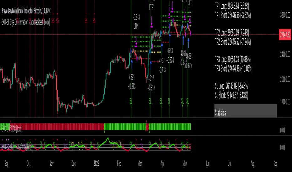
GKD-BT Giga Stacks Backtest [Loxx]Giga Kaleidoscope GKD-BT Giga Stacks Backtest is a Backtesting module included in Loxx's "Giga Kaleidoscope Modularized Trading System".
█ GKD-BT Giga Stacks Backtest
The Giga Stacks Backtest module allows users to perform backtesting on Long and Short signals from the confluence of GKD-B Baseline, GKD-C Confirmation, and GKD-V Volatility/Volume indicators. This module encompasses two types of backtests: Trading and Full. The Trading backtest permits users to evaluate individual trades, whether Long or Short, one at a time. Conversely, the Full backtest allows users to analyze either Longs or Shorts separately by toggling between them in the settings, enabling the examination of results for each signal type. The Trading backtest emulates actual trading conditions, while the Full backtest assesses all signals, regardless of being Long or Short.
Additionally, this backtest module provides the option to test using indicators with 1 to 3 take profits and 1 stop loss. The Trading backtest allows for the use of 1 to 3 take profits, while the Full backtest is limited to 1 take profit. The Trading backtest also offers the capability to apply a trailing take profit.
In terms of the percentage of trade removed at each take profit, this backtest module has the following hardcoded values:
Take profit 1: 50% of the trade is removed.
Take profit 2: 25% of the trade is removed.
Take profit 3: 25% of the trade is removed.
Stop loss: 100% of the trade is removed.
After each take profit is achieved, the stop loss level is adjusted. When take profit 1 is reached, the stop loss is moved to the entry point. Similarly, when take profit 2 is reached, the stop loss is shifted to take profit 1. The trailing take profit feature comes into play after take profit 2 or take profit 3, depending on the number of take profits selected in the settings. The trailing take profit is always activated on the final take profit when 2 or more take profits are chosen.
The backtest module also offers the capability to restrict by a specific date range, allowing for simulated forward testing based on past data. Additionally, users have the option to display or hide a trading panel that provides relevant information about the backtest, statistics, and the current trade. It is also possible to activate alerts and toggle sections of the trading panel on or off. On the chart, historical take profit and stop loss levels are represented by horizontal lines overlaid for reference.
To utilize this strategy, follow these steps (where "Stack XX" denotes the number of the Stack):
GKD-B Baseline Import: Import the value "Input into NEW GKD-BT Backtest" from the GKD-B Baseline module into the GKD-BT Giga Stacks Backtest module setting named "Stack XX: Import GKD-C, GKD-B, or GKD-V."
GKD-V Volatility/Volume Import: Import the value "Input into NEW GKD-BT Backtest" from the GKD-V Volatility/Volume module into the GKD-BT Giga Stacks Backtest module setting named "Stack XX: Import GKD-C, GKD-B, or GKD-V."
GKD-C Confirmation Import: 1) Adjust the "Confirmation Type" in the GKD-C Confirmation Indicator to "GKD New."; 2) Import the value "Input into NEW GKD-BT Backtest" from the GKD-C Confirmation module into the GKD-BT Giga Stacks Backtest module setting named "Stack XX: Import GKD-C, GKD-B, or GKD."
█ Giga Stacks Backtest Entries
Entries are generated form the confluence of up to six GKD-B Baseline, GKD-C Confirmation, and GKD-V Volatility/Volume indicators. Signals are generated when all Stacks reach uptrend or downtrend together.
Here's how this works. Assume we have the following Stacks and their respective trend on the current candle:
Stack 1 indicator is in uptreend
Stack 2 indicator is in downtrend
Stack 3 indicator is in uptreend
Stack 4 indicator is in uptreend
All stacks are in uptrend except for Stack 2. If Stack 2 reaches uptrend while Stacks 1, 3, and 4 stay in uptrend, then a long signal is generated. The last Stack to align with all other Stacks will generate a long or short signal.
█ Volatility Types Included
The GKD system utilizes volatility-based take profits and stop losses. Each take profit and stop loss is calculated as a multiple of volatility. Users can also adjust the multiplier values in the settings.
This module includes 17 types of volatility:
Close-to-Close
Parkinson
Garman-Klass
Rogers-Satchell
Yang-Zhang
Garman-Klass-Yang-Zhang
Exponential Weighted Moving Average
Standard Deviation of Log Returns
Pseudo GARCH(2,2)
Average True Range
True Range Double
Standard Deviation
Adaptive Deviation
Median Absolute Deviation
Efficiency-Ratio Adaptive ATR
Mean Absolute Deviation
Static Percent
Close-to-Close
Close-to-Close volatility is a classic and widely used volatility measure, sometimes referred to as historical volatility.
Volatility is an indicator of the speed of a stock price change. A stock with high volatility is one where the price changes rapidly and with a larger amplitude. The more volatile a stock is, the riskier it is.
Close-to-close historical volatility is calculated using only a stock's closing prices. It is the simplest volatility estimator. However, in many cases, it is not precise enough. Stock prices could jump significantly during a trading session and return to the opening value at the end. That means that a considerable amount of price information is not taken into account by close-to-close volatility.
Despite its drawbacks, Close-to-Close volatility is still useful in cases where the instrument doesn't have intraday prices. For example, mutual funds calculate their net asset values daily or weekly, and thus their prices are not suitable for more sophisticated volatility estimators.
Parkinson
Parkinson volatility is a volatility measure that uses the stock’s high and low price of the day.
The main difference between regular volatility and Parkinson volatility is that the latter uses high and low prices for a day, rather than only the closing price. This is useful as close-to-close prices could show little difference while large price movements could have occurred during the day. Thus, Parkinson's volatility is considered more precise and requires less data for calculation than close-to-close volatility.
One drawback of this estimator is that it doesn't take into account price movements after the market closes. Hence, it systematically undervalues volatility. This drawback is addressed in the Garman-Klass volatility estimator.
Garman-Klass
Garman-Klass is a volatility estimator that incorporates open, low, high, and close prices of a security.
Garman-Klass volatility extends Parkinson's volatility by taking into account the opening and closing prices. As markets are most active during the opening and closing of a trading session, it makes volatility estimation more accurate.
Garman and Klass also assumed that the process of price change follows a continuous diffusion process (Geometric Brownian motion). However, this assumption has several drawbacks. The method is not robust for opening jumps in price and trend movements.
Despite its drawbacks, the Garman-Klass estimator is still more effective than the basic formula since it takes into account not only the price at the beginning and end of the time interval but also intraday price extremes.
Researchers Rogers and Satchell have proposed a more efficient method for assessing historical volatility that takes into account price trends. See Rogers-Satchell Volatility for more detail.
Rogers-Satchell
Rogers-Satchell is an estimator for measuring the volatility of securities with an average return not equal to zero.
Unlike Parkinson and Garman-Klass estimators, Rogers-Satchell incorporates a drift term (mean return not equal to zero). As a result, it provides better volatility estimation when the underlying is trending.
The main disadvantage of this method is that it does not take into account price movements between trading sessions. This leads to an underestimation of volatility since price jumps periodically occur in the market precisely at the moments between sessions.
A more comprehensive estimator that also considers the gaps between sessions was developed based on the Rogers-Satchel formula in the 2000s by Yang-Zhang. See Yang Zhang Volatility for more detail.
Yang-Zhang
Yang Zhang is a historical volatility estimator that handles both opening jumps and the drift and has a minimum estimation error.
Yang-Zhang volatility can be thought of as a combination of the overnight (close-to-open volatility) and a weighted average of the Rogers-Satchell volatility and the day’s open-to-close volatility. It is considered to be 14 times more efficient than the close-to-close estimator.
Garman-Klass-Yang-Zhang
Garman-Klass-Yang-Zhang (GKYZ) volatility estimator incorporates the returns of open, high, low, and closing prices in its calculation.
GKYZ volatility estimator takes into account overnight jumps but not the trend, i.e., it assumes that the underlying asset follows a Geometric Brownian Motion (GBM) process with zero drift. Therefore, the GKYZ volatility estimator tends to overestimate the volatility when the drift is different from zero. However, for a GBM process, this estimator is eight times more efficient than the close-to-close volatility estimator.
Exponential Weighted Moving Average
The Exponentially Weighted Moving Average (EWMA) is a quantitative or statistical measure used to model or describe a time series. The EWMA is widely used in finance, with the main applications being technical analysis and volatility modeling.
The moving average is designed such that older observations are given lower weights. The weights decrease exponentially as the data point gets older – hence the name exponentially weighted.
The only decision a user of the EWMA must make is the parameter lambda. The parameter decides how important the current observation is in the calculation of the EWMA. The higher the value of lambda, the more closely the EWMA tracks the original time series.
Standard Deviation of Log Returns
This is the simplest calculation of volatility. It's the standard deviation of ln(close/close(1)).
Pseudo GARCH(2,2)
This is calculated using a short- and long-run mean of variance multiplied by ?.
?avg(var;M) + (1 ? ?) avg(var;N) = 2?var/(M+1-(M-1)L) + 2(1-?)var/(M+1-(M-1)L)
Solving for ? can be done by minimizing the mean squared error of estimation; that is, regressing L^-1var - avg(var; N) against avg(var; M) - avg(var; N) and using the resulting beta estimate as ?.
Average True Range
The average true range (ATR) is a technical analysis indicator, introduced by market technician J. Welles Wilder Jr. in his book New Concepts in Technical Trading Systems, that measures market volatility by decomposing the entire range of an asset price for that period.
The true range indicator is taken as the greatest of the following: current high less the current low; the absolute value of the current high less the previous close; and the absolute value of the current low less the previous close. The ATR is then a moving average, generally using 14 days, of the true ranges.
True Range Double
A special case of ATR that attempts to correct for volatility skew.
Standard Deviation
Standard deviation is a statistic that measures the dispersion of a dataset relative to its mean and is calculated as the square root of the variance. The standard deviation is calculated as the square root of variance by determining each data point's deviation relative to the mean. If the data points are further from the mean, there is a higher deviation within the data set; thus, the more spread out the data, the higher the standard deviation.
Adaptive Deviation
By definition, the Standard Deviation (STD, also represented by the Greek letter sigma ? or the Latin letter s) is a measure that is used to quantify the amount of variation or dispersion of a set of data values. In technical analysis, we usually use it to measure the level of current volatility.
Standard Deviation is based on Simple Moving Average calculation for mean value. This version of standard deviation uses the properties of EMA to calculate what can be called a new type of deviation, and since it is based on EMA, we can call it EMA deviation. Additionally, Perry Kaufman's efficiency ratio is used to make it adaptive (since all EMA type calculations are nearly perfect for adapting).
The difference when compared to the standard is significant--not just because of EMA usage, but the efficiency ratio makes it a "bit more logical" in very volatile market conditions.
Median Absolute Deviation
The median absolute deviation is a measure of statistical dispersion. Moreover, the MAD is a robust statistic, being more resilient to outliers in a data set than the standard deviation. In the standard deviation, the distances from the mean are squared, so large deviations are weighted more heavily, and thus outliers can heavily influence it. In the MAD, the deviations of a small number of outliers are irrelevant.
Because the MAD is a more robust estimator of scale than the sample variance or standard deviation, it works better with distributions without a mean or variance, such as the Cauchy distribution.
Efficiency-Ratio Adaptive ATR
Average True Range (ATR) is a widely used indicator for many occasions in technical analysis. It is calculated as the RMA of the true range. This version adds a "twist": it uses Perry Kaufman's Efficiency Ratio to calculate adaptive true range.
Mean Absolute Deviation
The mean absolute deviation (MAD) is a measure of variability that indicates the average distance between observations and their mean. MAD uses the original units of the data, which simplifies interpretation. Larger values signify that the data points spread out further from the average. Conversely, lower values correspond to data points bunching closer to it. The mean absolute deviation is also known as the mean deviation and average absolute deviation.
This definition of the mean absolute deviation sounds similar to the standard deviation (SD). While both measure variability, they have different calculations. In recent years, some proponents of MAD have suggested that it replace the SD as the primary measure because it is a simpler concept that better fits real life.
Static Percent
Static Percent allows the user to insert their own constant percent that will then be used to create take profits and stoploss
█ Giga Kaleidoscope Modularized Trading System
Core components of an NNFX algorithmic trading strategy
The NNFX algorithm is built on the principles of trend, momentum, and volatility. There are six core components in the NNFX trading algorithm:
1. Volatility - price volatility; e.g., Average True Range, True Range Double, Close-to-Close, etc.
2. Baseline - a moving average to identify price trend
3. Confirmation 1 - a technical indicator used to identify trends
4. Confirmation 2 - a technical indicator used to identify trends
5. Continuation - a technical indicator used to identify trends
6. Volatility/Volume - a technical indicator used to identify volatility/volume breakouts/breakdown
7. Exit - a technical indicator used to determine when a trend is exhausted
What is Volatility in the NNFX trading system?
In the NNFX (No Nonsense Forex) trading system, ATR (Average True Range) is typically used to measure the volatility of an asset. It is used as a part of the system to help determine the appropriate stop loss and take profit levels for a trade. ATR is calculated by taking the average of the true range values over a specified period.
True range is calculated as the maximum of the following values:
-Current high minus the current low
-Absolute value of the current high minus the previous close
-Absolute value of the current low minus the previous close
ATR is a dynamic indicator that changes with changes in volatility. As volatility increases, the value of ATR increases, and as volatility decreases, the value of ATR decreases. By using ATR in NNFX system, traders can adjust their stop loss and take profit levels according to the volatility of the asset being traded. This helps to ensure that the trade is given enough room to move, while also minimizing potential losses.
Other types of volatility include True Range Double (TRD), Close-to-Close, and Garman-Klass
What is a Baseline indicator?
The baseline is essentially a moving average, and is used to determine the overall direction of the market.
The baseline in the NNFX system is used to filter out trades that are not in line with the long-term trend of the market. The baseline is plotted on the chart along with other indicators, such as the Moving Average (MA), the Relative Strength Index (RSI), and the Average True Range (ATR).
Trades are only taken when the price is in the same direction as the baseline. For example, if the baseline is sloping upwards, only long trades are taken, and if the baseline is sloping downwards, only short trades are taken. This approach helps to ensure that trades are in line with the overall trend of the market, and reduces the risk of entering trades that are likely to fail.
By using a baseline in the NNFX system, traders can have a clear reference point for determining the overall trend of the market, and can make more informed trading decisions. The baseline helps to filter out noise and false signals, and ensures that trades are taken in the direction of the long-term trend.
What is a Confirmation indicator?
Confirmation indicators are technical indicators that are used to confirm the signals generated by primary indicators. Primary indicators are the core indicators used in the NNFX system, such as the Average True Range (ATR), the Moving Average (MA), and the Relative Strength Index (RSI).
The purpose of the confirmation indicators is to reduce false signals and improve the accuracy of the trading system. They are designed to confirm the signals generated by the primary indicators by providing additional information about the strength and direction of the trend.
Some examples of confirmation indicators that may be used in the NNFX system include the Bollinger Bands, the MACD (Moving Average Convergence Divergence), and the MACD Oscillator. These indicators can provide information about the volatility, momentum, and trend strength of the market, and can be used to confirm the signals generated by the primary indicators.
In the NNFX system, confirmation indicators are used in combination with primary indicators and other filters to create a trading system that is robust and reliable. By using multiple indicators to confirm trading signals, the system aims to reduce the risk of false signals and improve the overall profitability of the trades.
What is a Continuation indicator?
In the NNFX (No Nonsense Forex) trading system, a continuation indicator is a technical indicator that is used to confirm a current trend and predict that the trend is likely to continue in the same direction. A continuation indicator is typically used in conjunction with other indicators in the system, such as a baseline indicator, to provide a comprehensive trading strategy.
What is a Volatility/Volume indicator?
Volume indicators, such as the On Balance Volume (OBV), the Chaikin Money Flow (CMF), or the Volume Price Trend (VPT), are used to measure the amount of buying and selling activity in a market. They are based on the trading volume of the market, and can provide information about the strength of the trend. In the NNFX system, volume indicators are used to confirm trading signals generated by the Moving Average and the Relative Strength Index. Volatility indicators include Average Direction Index, Waddah Attar, and Volatility Ratio. In the NNFX trading system, volatility is a proxy for volume and vice versa.
By using volume indicators as confirmation tools, the NNFX trading system aims to reduce the risk of false signals and improve the overall profitability of trades. These indicators can provide additional information about the market that is not captured by the primary indicators, and can help traders to make more informed trading decisions. In addition, volume indicators can be used to identify potential changes in market trends and to confirm the strength of price movements.
What is an Exit indicator?
The exit indicator is used in conjunction with other indicators in the system, such as the Moving Average (MA), the Relative Strength Index (RSI), and the Average True Range (ATR), to provide a comprehensive trading strategy.
The exit indicator in the NNFX system can be any technical indicator that is deemed effective at identifying optimal exit points. Examples of exit indicators that are commonly used include the Parabolic SAR, the Average Directional Index (ADX), and the Chandelier Exit.
The purpose of the exit indicator is to identify when a trend is likely to reverse or when the market conditions have changed, signaling the need to exit a trade. By using an exit indicator, traders can manage their risk and prevent significant losses.
In the NNFX system, the exit indicator is used in conjunction with a stop loss and a take profit order to maximize profits and minimize losses. The stop loss order is used to limit the amount of loss that can be incurred if the trade goes against the trader, while the take profit order is used to lock in profits when the trade is moving in the trader's favor.
Overall, the use of an exit indicator in the NNFX trading system is an important component of a comprehensive trading strategy. It allows traders to manage their risk effectively and improve the profitability of their trades by exiting at the right time.
How does Loxx's GKD (Giga Kaleidoscope Modularized Trading System) implement the NNFX algorithm outlined above?
Loxx's GKD v2.0 system has five types of modules (indicators/strategies). These modules are:
1. GKD-BT - Backtesting module (Volatility, Number 1 in the NNFX algorithm)
2. GKD-B - Baseline module (Baseline and Volatility/Volume, Numbers 1 and 2 in the NNFX algorithm)
3. GKD-C - Confirmation 1/2 and Continuation module (Confirmation 1/2 and Continuation, Numbers 3, 4, and 5 in the NNFX algorithm)
4. GKD-V - Volatility/Volume module (Confirmation 1/2, Number 6 in the NNFX algorithm)
5. GKD-E - Exit module (Exit, Number 7 in the NNFX algorithm)
(additional module types will added in future releases)
Each module interacts with every module by passing data to A backtest module wherein the various components of the GKD system are combined to create a trading signal.
That is, the Baseline indicator passes its data to Volatility/Volume. The Volatility/Volume indicator passes its values to the Confirmation 1 indicator. The Confirmation 1 indicator passes its values to the Confirmation 2 indicator. The Confirmation 2 indicator passes its values to the Continuation indicator. The Continuation indicator passes its values to the Exit indicator, and finally, the Exit indicator passes its values to the Backtest strategy.
This chaining of indicators requires that each module conform to Loxx's GKD protocol, therefore allowing for the testing of every possible combination of technical indicators that make up the six components of the NNFX algorithm.
What does the application of the GKD trading system look like?
Example trading system:
Backtest: Stacks Backtest
Baseline: Hull Moving Average
Volatility/Volume: Hurst Exponent
Confirmation 1: Vorext
Confirmation 2: Coppock Curve
Continuation: Fisher Transform
Exit: Rex Oscillator
Each GKD indicator is denoted with a module identifier of either: GKD-BT, GKD-B, GKD-C, GKD-V, or GKD-E. This allows traders to understand to which module each indicator belongs and where each indicator fits into the GKD system.

GKD-BT Full Giga Kaleidoscope Backtest [Loxx]Giga Kaleidoscope GKD-BT Full Giga Kaleidoscope Backtest is a Backtesting module included in Loxx's "Giga Kaleidoscope Modularized Trading System".
█ GKD-BT Full Giga Kaleidoscope Backtest
The Full Giga Kaleidoscope Backtest module enables users to backtest Full GKD Long and Short signals, allowing the creation of a comprehensive NNFX trading system consisting of two confirmation indicators, a baseline, a measure of volatility/volume, and continuations.
This module offers two types of backtests: Trading and Full. The Trading backtest allows users to evaluate individual Long and Short trades one by one. On the other hand, the Full backtest enables the analysis of Longs or Shorts separately by toggling between them in the settings, providing insights into the results for each signal type. The Trading backtest simulates actual trading conditions, while the Full backtest evaluates all signals regardless of their Long or Short nature.
Additionally, the backtest module allows testing with 1 to 3 take profits and 1 stop loss. The Trading backtest supports 1 to 3 take profits, while the Full backtest is limited to 1 take profit. The Trading backtest also includes a trailing take profit feature.
Regarding the percentage of trade removed at each take profit, the backtest module incorporates the following predefined values:
Take profit 1: 50% of the trade is removed.
Take profit 2: 25% of the trade is removed.
Take profit 3: 25% of the trade is removed.
Stop loss: 100% of the trade is removed.
After achieving each take profit, the stop loss level is adjusted accordingly. When take profit 1 is reached, the stop loss is moved to the entry point. Similarly, when take profit 2 is reached, the stop loss is shifted to take profit 1. The trailing take profit feature comes into effect after take profit 2 or take profit 3, depending on the number of take profits selected in the settings. The trailing take profit is always activated on the final take profit when 2 or more take profits are chosen.
The backtest module also provides the option to restrict testing to a specific date range, allowing for simulated forward testing using past data. Additionally, users can choose to display or hide a trading panel that provides relevant information about the backtest, statistics, and the current trade. It is also possible to activate alerts and toggle sections of the trading panel on or off. Historical take profit and stop loss levels are displayed as overlaid horizontal lines on the chart for reference.
To utilize this strategy, follow these steps:
1. GKD-B Baseline Import: Import the value "Input into NEW GKD-BT Backtest" from the GKD-B Baseline module into the GKD-BT Full Giga Kaleidoscope Backtest module setting named "Import GKD-B Baseline."
2. GKD-V Volatility/Volume Import: Import the value "Input into NEW GKD-BT Backtest" from the GKD-V Volatility/Volume module into the GKD-BT Full Giga Kaleidoscope Backtest module setting named "Import GKD-V Volatility/Volume."
3. Adjust the "Confirmation 1 Type" in the GKD-C Confirmation Indicator to "GKD New."
4. GKD-C Confirmation 1 Import: Import the value "Input into NEW GKD-BT Backtest" from the GKD-C Confirmation 1 module into the GKD-BT Full Giga Kaleidoscope Backtest module setting named "Import GKD-C Confirmation 1."
5. Adjust the "Confirmation 2 Type" in the GKD-C Confirmation 2 Indicator to "GKD New."
6. GKD-C Confirmation 2 Import: Import the value "Input into NEW GKD-BT Backtest" from the GKD-C Confirmation 2 module into the GKD-BT Full Giga Kaleidoscope Backtest module setting named "Import GKD-C Confirmation 2."
7. Adjust the "Confirmation Type" in the GKD-C Continuation Indicator to "GKD New."
8. GKD-C Continuation Import: Import the value "Input into NEW GKD-BT Backtest" from the GKD-C Continuation module into the GKD-BT Full Giga Kaleidoscope Backtest module setting named "Import GKD-C Confirmation."
The GKD system utilizes volatility-based take profits and stop losses, where each take profit and stop loss is calculated as a multiple of volatility. Users have the flexibility to adjust the multiplier values in the settings to suit their preferences.
In a future update, the Full Giga Kaleidoscope Backtest module will include the option to incorporate a GKD-E Exit indicator, completing the full trading strategy.
█ Full Giga Kaleidoscope Backtest Entries
Within this module, there are ten distinct types of entries available, which are outlined below:
Standard Entry
1-Candle Standard Entry
Baseline Entry
1-Candle Baseline Entry
Volatility/Volume Entry
1-Candle Volatility/Volume Entry
Confirmation 2 Entry
1-Candle Confirmation 2 Entry
PullBack Entry
Continuation Entry
Each of these entry types can generate either long or short signals, resulting in a total of 20 signal variations. The user has the flexibility to enable or disable specific entry types and choose which qualifying rules within each entry type are applied to price to determine the final long or short signal.
The following section provides an overview of the various entry types and their corresponding qualifying rules:
Standard Entry
1. GKD-C Confirmation gives signal
2. Baseline agrees
3. Price inside Goldie Locks Zone Minimum
4. Price inside Goldie Locks Zone Maximum
5. Confirmation 2 agrees
6. Volatility/Volume agrees
1-Candle Standard Entry
1a. GKD-C Confirmation gives signal
2a. Baseline agrees
3a. Price inside Goldie Locks Zone Minimum
4a. Price inside Goldie Locks Zone Maximum
Next Candle
1b. Price retraced
2b. Baseline agrees
3b. Confirmation 1 agrees
4b. Confirmation 2 agrees
5b. Volatility/Volume agrees
Baseline Entry
1. GKD-B Basline gives signal
2. Confirmation 1 agrees
3. Price inside Goldie Locks Zone Minimum
4. Price inside Goldie Locks Zone Maximum
5. Confirmation 2 agrees
6. Volatility/Volume agrees
7. Confirmation 1 signal was less than 'Maximum Allowable PSBC Bars Back' prior
1-Candle Baseline Entry
1a. GKD-B Baseline gives signal
2a. Confirmation 1 agrees
3a. Price inside Goldie Locks Zone Minimum
4a. Price inside Goldie Locks Zone Maximum
5a. Confirmation 1 signal was less than 'Maximum Allowable PSBC Bars Back' prior
Next Candle
1b. Price retraced
2b. Baseline agrees
3b. Confirmation 1 agrees
4b. Confirmation 2 agrees
5b. Volatility/Volume agrees
Volatility/Volume Entry
1. GKD-V Volatility/Volume gives signal
2. Confirmation 1 agrees
3. Price inside Goldie Locks Zone Minimum
4. Price inside Goldie Locks Zone Maximum
5. Confirmation 2 agrees
6. Baseline agrees
7. Confirmation 1 signal was less than 7 candles prior
1-Candle Volatility/Volume Entry
1a. GKD-V Volatility/Volume gives signal
2a. Confirmation 1 agrees
3a. Price inside Goldie Locks Zone Minimum
4a. Price inside Goldie Locks Zone Maximum
5a. Confirmation 1 signal was less than 'Maximum Allowable PSVVC Bars Back' prior
Next Candle
1b. Price retraced
2b. Volatility/Volume agrees
3b. Confirmation 1 agrees
4b. Confirmation 2 agrees
5b. Baseline agrees
Confirmation 2 Entry
1. GKD-C Confirmation 2 gives signal
2. Confirmation 1 agrees
3. Price inside Goldie Locks Zone Minimum
4. Price inside Goldie Locks Zone Maximum
5. Volatility/Volume agrees
6. Baseline agrees
7. Confirmation 1 signal was less than 7 candles prior
1-Candle Confirmation 2 Entry
1a. GKD-C Confirmation 2 gives signal
2a. Confirmation 1 agrees
3a. Price inside Goldie Locks Zone Minimum
4a. Price inside Goldie Locks Zone Maximum
5a. Confirmation 1 signal was less than 'Maximum Allowable PSC2C Bars Back' prior
Next Candle
1b. Price retraced
2b. Confirmation 2 agrees
3b. Confirmation 1 agrees
4b. Volatility/Volume agrees
5b. Baseline agrees
PullBack Entry
1a. GKD-B Baseline gives signal
2a. Confirmation 1 agrees
3a. Price is beyond 1.0x Volatility of Baseline
Next Candle
1b. Price inside Goldie Locks Zone Minimum
2b. Price inside Goldie Locks Zone Maximum
3b. Confirmation 1 agrees
4b. Confirmation 2 agrees
5b. Volatility/Volume agrees
Continuation Entry
1. Standard Entry, 1-Candle Standard Entry, Baseline Entry, 1-Candle Baseline Entry, Volatility/Volume Entry, 1-Candle Volatility/Volume Entry, Confirmation 2 Entry, 1-Candle Confirmation 2 Entry, or Pullback entry triggered previously
2. Baseline hasn't crossed since entry signal trigger
4. Confirmation 1 agrees
5. Baseline agrees
6. Confirmation 2 agrees
█ Volatility Types Included
This module includes 17 types of volatility:
Close-to-Close
Parkinson
Garman-Klass
Rogers-Satchell
Yang-Zhang
Garman-Klass-Yang-Zhang
Exponential Weighted Moving Average
Standard Deviation of Log Returns
Pseudo GARCH(2,2)
Average True Range
True Range Double
Standard Deviation
Adaptive Deviation
Median Absolute Deviation
Efficiency-Ratio Adaptive ATR
Mean Absolute Deviation
Static Percent
Close-to-Close
Close-to-Close volatility is a classic and widely used volatility measure, sometimes referred to as historical volatility.
Volatility is an indicator of the speed of a stock price change. A stock with high volatility is one where the price changes rapidly and with a larger amplitude. The more volatile a stock is, the riskier it is.
Close-to-close historical volatility is calculated using only a stock's closing prices. It is the simplest volatility estimator. However, in many cases, it is not precise enough. Stock prices could jump significantly during a trading session and return to the opening value at the end. That means that a considerable amount of price information is not taken into account by close-to-close volatility.
Despite its drawbacks, Close-to-Close volatility is still useful in cases where the instrument doesn't have intraday prices. For example, mutual funds calculate their net asset values daily or weekly, and thus their prices are not suitable for more sophisticated volatility estimators.
Parkinson
Parkinson volatility is a volatility measure that uses the stock’s high and low price of the day.
The main difference between regular volatility and Parkinson volatility is that the latter uses high and low prices for a day, rather than only the closing price. This is useful as close-to-close prices could show little difference while large price movements could have occurred during the day. Thus, Parkinson's volatility is considered more precise and requires less data for calculation than close-to-close volatility.
One drawback of this estimator is that it doesn't take into account price movements after the market closes. Hence, it systematically undervalues volatility. This drawback is addressed in the Garman-Klass volatility estimator.
Garman-Klass
Garman-Klass is a volatility estimator that incorporates open, low, high, and close prices of a security.
Garman-Klass volatility extends Parkinson's volatility by taking into account the opening and closing prices. As markets are most active during the opening and closing of a trading session, it makes volatility estimation more accurate.
Garman and Klass also assumed that the process of price change follows a continuous diffusion process (Geometric Brownian motion). However, this assumption has several drawbacks. The method is not robust for opening jumps in price and trend movements.
Despite its drawbacks, the Garman-Klass estimator is still more effective than the basic formula since it takes into account not only the price at the beginning and end of the time interval but also intraday price extremes.
Researchers Rogers and Satchell have proposed a more efficient method for assessing historical volatility that takes into account price trends. See Rogers-Satchell Volatility for more detail.
Rogers-Satchell
Rogers-Satchell is an estimator for measuring the volatility of securities with an average return not equal to zero.
Unlike Parkinson and Garman-Klass estimators, Rogers-Satchell incorporates a drift term (mean return not equal to zero). As a result, it provides better volatility estimation when the underlying is trending.
The main disadvantage of this method is that it does not take into account price movements between trading sessions. This leads to an underestimation of volatility since price jumps periodically occur in the market precisely at the moments between sessions.
A more comprehensive estimator that also considers the gaps between sessions was developed based on the Rogers-Satchel formula in the 2000s by Yang-Zhang. See Yang Zhang Volatility for more detail.
Yang-Zhang
Yang Zhang is a historical volatility estimator that handles both opening jumps and the drift and has a minimum estimation error.
Yang-Zhang volatility can be thought of as a combination of the overnight (close-to-open volatility) and a weighted average of the Rogers-Satchell volatility and the day’s open-to-close volatility. It is considered to be 14 times more efficient than the close-to-close estimator.
Garman-Klass-Yang-Zhang
Garman-Klass-Yang-Zhang (GKYZ) volatility estimator incorporates the returns of open, high, low, and closing prices in its calculation.
GKYZ volatility estimator takes into account overnight jumps but not the trend, i.e., it assumes that the underlying asset follows a Geometric Brownian Motion (GBM) process with zero drift. Therefore, the GKYZ volatility estimator tends to overestimate the volatility when the drift is different from zero. However, for a GBM process, this estimator is eight times more efficient than the close-to-close volatility estimator.
Exponential Weighted Moving Average
The Exponentially Weighted Moving Average (EWMA) is a quantitative or statistical measure used to model or describe a time series. The EWMA is widely used in finance, with the main applications being technical analysis and volatility modeling.
The moving average is designed such that older observations are given lower weights. The weights decrease exponentially as the data point gets older – hence the name exponentially weighted.
The only decision a user of the EWMA must make is the parameter lambda. The parameter decides how important the current observation is in the calculation of the EWMA. The higher the value of lambda, the more closely the EWMA tracks the original time series.
Standard Deviation of Log Returns
This is the simplest calculation of volatility. It's the standard deviation of ln(close/close(1)).
Pseudo GARCH(2,2)
This is calculated using a short- and long-run mean of variance multiplied by ?.
?avg(var;M) + (1 ? ?) avg(var;N) = 2?var/(M+1-(M-1)L) + 2(1-?)var/(M+1-(M-1)L)
Solving for ? can be done by minimizing the mean squared error of estimation; that is, regressing L^-1var - avg(var; N) against avg(var; M) - avg(var; N) and using the resulting beta estimate as ?.
Average True Range
The average true range (ATR) is a technical analysis indicator, introduced by market technician J. Welles Wilder Jr. in his book New Concepts in Technical Trading Systems, that measures market volatility by decomposing the entire range of an asset price for that period.
The true range indicator is taken as the greatest of the following: current high less the current low; the absolute value of the current high less the previous close; and the absolute value of the current low less the previous close. The ATR is then a moving average, generally using 14 days, of the true ranges.
True Range Double
A special case of ATR that attempts to correct for volatility skew.
Standard Deviation
Standard deviation is a statistic that measures the dispersion of a dataset relative to its mean and is calculated as the square root of the variance. The standard deviation is calculated as the square root of variance by determining each data point's deviation relative to the mean. If the data points are further from the mean, there is a higher deviation within the data set; thus, the more spread out the data, the higher the standard deviation.
Adaptive Deviation
By definition, the Standard Deviation (STD, also represented by the Greek letter sigma ? or the Latin letter s) is a measure that is used to quantify the amount of variation or dispersion of a set of data values. In technical analysis, we usually use it to measure the level of current volatility.
Standard Deviation is based on Simple Moving Average calculation for mean value. This version of standard deviation uses the properties of EMA to calculate what can be called a new type of deviation, and since it is based on EMA, we can call it EMA deviation. Additionally, Perry Kaufman's efficiency ratio is used to make it adaptive (since all EMA type calculations are nearly perfect for adapting).
The difference when compared to the standard is significant--not just because of EMA usage, but the efficiency ratio makes it a "bit more logical" in very volatile market conditions.
Median Absolute Deviation
The median absolute deviation is a measure of statistical dispersion. Moreover, the MAD is a robust statistic, being more resilient to outliers in a data set than the standard deviation. In the standard deviation, the distances from the mean are squared, so large deviations are weighted more heavily, and thus outliers can heavily influence it. In the MAD, the deviations of a small number of outliers are irrelevant.
Because the MAD is a more robust estimator of scale than the sample variance or standard deviation, it works better with distributions without a mean or variance, such as the Cauchy distribution.
Efficiency-Ratio Adaptive ATR
Average True Range (ATR) is a widely used indicator for many occasions in technical analysis. It is calculated as the RMA of the true range. This version adds a "twist": it uses Perry Kaufman's Efficiency Ratio to calculate adaptive true range.
Mean Absolute Deviation
The mean absolute deviation (MAD) is a measure of variability that indicates the average distance between observations and their mean. MAD uses the original units of the data, which simplifies interpretation. Larger values signify that the data points spread out further from the average. Conversely, lower values correspond to data points bunching closer to it. The mean absolute deviation is also known as the mean deviation and average absolute deviation.
This definition of the mean absolute deviation sounds similar to the standard deviation (SD). While both measure variability, they have different calculations. In recent years, some proponents of MAD have suggested that it replace the SD as the primary measure because it is a simpler concept that better fits real life.
Static Percent
Static Percent allows the user to insert their own constant percent that will then be used to create take profits and stoploss
█ Giga Kaleidoscope Modularized Trading System
Core components of an NNFX algorithmic trading strategy
The NNFX algorithm is built on the principles of trend, momentum, and volatility. There are six core components in the NNFX trading algorithm:
1. Volatility - price volatility; e.g., Average True Range, True Range Double, Close-to-Close, etc.
2. Baseline - a moving average to identify price trend
3. Confirmation 1 - a technical indicator used to identify trends
4. Confirmation 2 - a technical indicator used to identify trends
5. Continuation - a technical indicator used to identify trends
6. Volatility/Volume - a technical indicator used to identify volatility/volume breakouts/breakdown
7. Exit - a technical indicator used to determine when a trend is exhausted
What is Volatility in the NNFX trading system?
In the NNFX (No Nonsense Forex) trading system, ATR (Average True Range) is typically used to measure the volatility of an asset. It is used as a part of the system to help determine the appropriate stop loss and take profit levels for a trade. ATR is calculated by taking the average of the true range values over a specified period.
True range is calculated as the maximum of the following values:
-Current high minus the current low
-Absolute value of the current high minus the previous close
-Absolute value of the current low minus the previous close
ATR is a dynamic indicator that changes with changes in volatility. As volatility increases, the value of ATR increases, and as volatility decreases, the value of ATR decreases. By using ATR in NNFX system, traders can adjust their stop loss and take profit levels according to the volatility of the asset being traded. This helps to ensure that the trade is given enough room to move, while also minimizing potential losses.
Other types of volatility include True Range Double (TRD), Close-to-Close, and Garman-Klass
What is a Baseline indicator?
The baseline is essentially a moving average, and is used to determine the overall direction of the market.
The baseline in the NNFX system is used to filter out trades that are not in line with the long-term trend of the market. The baseline is plotted on the chart along with other indicators, such as the Moving Average (MA), the Relative Strength Index (RSI), and the Average True Range (ATR).
Trades are only taken when the price is in the same direction as the baseline. For example, if the baseline is sloping upwards, only long trades are taken, and if the baseline is sloping downwards, only short trades are taken. This approach helps to ensure that trades are in line with the overall trend of the market, and reduces the risk of entering trades that are likely to fail.
By using a baseline in the NNFX system, traders can have a clear reference point for determining the overall trend of the market, and can make more informed trading decisions. The baseline helps to filter out noise and false signals, and ensures that trades are taken in the direction of the long-term trend.
What is a Confirmation indicator?
Confirmation indicators are technical indicators that are used to confirm the signals generated by primary indicators. Primary indicators are the core indicators used in the NNFX system, such as the Average True Range (ATR), the Moving Average (MA), and the Relative Strength Index (RSI).
The purpose of the confirmation indicators is to reduce false signals and improve the accuracy of the trading system. They are designed to confirm the signals generated by the primary indicators by providing additional information about the strength and direction of the trend.
Some examples of confirmation indicators that may be used in the NNFX system include the Bollinger Bands, the MACD (Moving Average Convergence Divergence), and the MACD Oscillator. These indicators can provide information about the volatility, momentum, and trend strength of the market, and can be used to confirm the signals generated by the primary indicators.
In the NNFX system, confirmation indicators are used in combination with primary indicators and other filters to create a trading system that is robust and reliable. By using multiple indicators to confirm trading signals, the system aims to reduce the risk of false signals and improve the overall profitability of the trades.
What is a Continuation indicator?
In the NNFX (No Nonsense Forex) trading system, a continuation indicator is a technical indicator that is used to confirm a current trend and predict that the trend is likely to continue in the same direction. A continuation indicator is typically used in conjunction with other indicators in the system, such as a baseline indicator, to provide a comprehensive trading strategy.
What is a Volatility/Volume indicator?
Volume indicators, such as the On Balance Volume (OBV), the Chaikin Money Flow (CMF), or the Volume Price Trend (VPT), are used to measure the amount of buying and selling activity in a market. They are based on the trading volume of the market, and can provide information about the strength of the trend. In the NNFX system, volume indicators are used to confirm trading signals generated by the Moving Average and the Relative Strength Index. Volatility indicators include Average Direction Index, Waddah Attar, and Volatility Ratio. In the NNFX trading system, volatility is a proxy for volume and vice versa.
By using volume indicators as confirmation tools, the NNFX trading system aims to reduce the risk of false signals and improve the overall profitability of trades. These indicators can provide additional information about the market that is not captured by the primary indicators, and can help traders to make more informed trading decisions. In addition, volume indicators can be used to identify potential changes in market trends and to confirm the strength of price movements.
What is an Exit indicator?
The exit indicator is used in conjunction with other indicators in the system, such as the Moving Average (MA), the Relative Strength Index (RSI), and the Average True Range (ATR), to provide a comprehensive trading strategy.
The exit indicator in the NNFX system can be any technical indicator that is deemed effective at identifying optimal exit points. Examples of exit indicators that are commonly used include the Parabolic SAR, the Average Directional Index (ADX), and the Chandelier Exit.
The purpose of the exit indicator is to identify when a trend is likely to reverse or when the market conditions have changed, signaling the need to exit a trade. By using an exit indicator, traders can manage their risk and prevent significant losses.
In the NNFX system, the exit indicator is used in conjunction with a stop loss and a take profit order to maximize profits and minimize losses. The stop loss order is used to limit the amount of loss that can be incurred if the trade goes against the trader, while the take profit order is used to lock in profits when the trade is moving in the trader's favor.
Overall, the use of an exit indicator in the NNFX trading system is an important component of a comprehensive trading strategy. It allows traders to manage their risk effectively and improve the profitability of their trades by exiting at the right time.
How does Loxx's GKD (Giga Kaleidoscope Modularized Trading System) implement the NNFX algorithm outlined above?
Loxx's GKD v2.0 system has five types of modules (indicators/strategies). These modules are:
1. GKD-BT - Backtesting module (Volatility, Number 1 in the NNFX algorithm)
2. GKD-B - Baseline module (Baseline and Volatility/Volume, Numbers 1 and 2 in the NNFX algorithm)
3. GKD-C - Confirmation 1/2 and Continuation module (Confirmation 1/2 and Continuation, Numbers 3, 4, and 5 in the NNFX algorithm)
4. GKD-V - Volatility/Volume module (Confirmation 1/2, Number 6 in the NNFX algorithm)
5. GKD-E - Exit module (Exit, Number 7 in the NNFX algorithm)
(additional module types will added in future releases)
Each module interacts with every module by passing data to A backtest module wherein the various components of the GKD system are combined to create a trading signal.
That is, the Baseline indicator passes its data to Volatility/Volume. The Volatility/Volume indicator passes its values to the Confirmation 1 indicator. The Confirmation 1 indicator passes its values to the Confirmation 2 indicator. The Confirmation 2 indicator passes its values to the Continuation indicator. The Continuation indicator passes its values to the Exit indicator, and finally, the Exit indicator passes its values to the Backtest strategy.
This chaining of indicators requires that each module conform to Loxx's GKD protocol, therefore allowing for the testing of every possible combination of technical indicators that make up the six components of the NNFX algorithm.
What does the application of the GKD trading system look like?
Example trading system:
Backtest: Full Giga Kaleidoscope Backtest as shown on the chart above
Baseline: Hull Moving Average as shown on the chart above
Volatility/Volume: Hurst Exponent as shown on the chart above
Confirmation 1: Vorext as shown on the chart above
Confirmation 2: Coppock Curve as shown on the chart above
Continuation: Fisher Transform as shown on the chart above
Exit: Rex Oscillator
Each GKD indicator is denoted with a module identifier of either: GKD-BT, GKD-B, GKD-C, GKD-V, or GKD-E. This allows traders to understand to which module each indicator belongs and where each indicator fits into the GKD system.
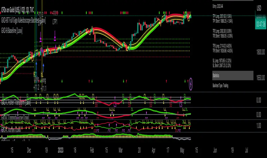
Machine Learning: Lorentzian Classification█ OVERVIEW
A Lorentzian Distance Classifier (LDC) is a Machine Learning classification algorithm capable of categorizing historical data from a multi-dimensional feature space. This indicator demonstrates how Lorentzian Classification can also be used to predict the direction of future price movements when used as the distance metric for a novel implementation of an Approximate Nearest Neighbors (ANN) algorithm.
█ BACKGROUND
In physics, Lorentzian space is perhaps best known for its role in describing the curvature of space-time in Einstein's theory of General Relativity (2). Interestingly, however, this abstract concept from theoretical physics also has tangible real-world applications in trading.
Recently, it was hypothesized that Lorentzian space was also well-suited for analyzing time-series data (4), (5). This hypothesis has been supported by several empirical studies that demonstrate that Lorentzian distance is more robust to outliers and noise than the more commonly used Euclidean distance (1), (3), (6). Furthermore, Lorentzian distance was also shown to outperform dozens of other highly regarded distance metrics, including Manhattan distance, Bhattacharyya similarity, and Cosine similarity (1), (3). Outside of Dynamic Time Warping based approaches, which are unfortunately too computationally intensive for PineScript at this time, the Lorentzian Distance metric consistently scores the highest mean accuracy over a wide variety of time series data sets (1).
Euclidean distance is commonly used as the default distance metric for NN-based search algorithms, but it may not always be the best choice when dealing with financial market data. This is because financial market data can be significantly impacted by proximity to major world events such as FOMC Meetings and Black Swan events. This event-based distortion of market data can be framed as similar to the gravitational warping caused by a massive object on the space-time continuum. For financial markets, the analogous continuum that experiences warping can be referred to as "price-time".
Below is a side-by-side comparison of how neighborhoods of similar historical points appear in three-dimensional Euclidean Space and Lorentzian Space:
This figure demonstrates how Lorentzian space can better accommodate the warping of price-time since the Lorentzian distance function compresses the Euclidean neighborhood in such a way that the new neighborhood distribution in Lorentzian space tends to cluster around each of the major feature axes in addition to the origin itself. This means that, even though some nearest neighbors will be the same regardless of the distance metric used, Lorentzian space will also allow for the consideration of historical points that would otherwise never be considered with a Euclidean distance metric.
Intuitively, the advantage inherent in the Lorentzian distance metric makes sense. For example, it is logical that the price action that occurs in the hours after Chairman Powell finishes delivering a speech would resemble at least some of the previous times when he finished delivering a speech. This may be true regardless of other factors, such as whether or not the market was overbought or oversold at the time or if the macro conditions were more bullish or bearish overall. These historical reference points are extremely valuable for predictive models, yet the Euclidean distance metric would miss these neighbors entirely, often in favor of irrelevant data points from the day before the event. By using Lorentzian distance as a metric, the ML model is instead able to consider the warping of price-time caused by the event and, ultimately, transcend the temporal bias imposed on it by the time series.
For more information on the implementation details of the Approximate Nearest Neighbors (ANN) algorithm used in this indicator, please refer to the detailed comments in the source code.
█ HOW TO USE
Below is an explanatory breakdown of the different parts of this indicator as it appears in the interface:
Below is an explanation of the different settings for this indicator:
General Settings:
Source - This has a default value of "hlc3" and is used to control the input data source.
Neighbors Count - This has a default value of 8, a minimum value of 1, a maximum value of 100, and a step of 1. It is used to control the number of neighbors to consider.
Max Bars Back - This has a default value of 2000.
Feature Count - This has a default value of 5, a minimum value of 2, and a maximum value of 5. It controls the number of features to use for ML predictions.
Color Compression - This has a default value of 1, a minimum value of 1, and a maximum value of 10. It is used to control the compression factor for adjusting the intensity of the color scale.
Show Exits - This has a default value of false. It controls whether to show the exit threshold on the chart.
Use Dynamic Exits - This has a default value of false. It is used to control whether to attempt to let profits ride by dynamically adjusting the exit threshold based on kernel regression.
Feature Engineering Settings:
Note: The Feature Engineering section is for fine-tuning the features used for ML predictions. The default values are optimized for the 4H to 12H timeframes for most charts, but they should also work reasonably well for other timeframes. By default, the model can support features that accept two parameters (Parameter A and Parameter B, respectively). Even though there are only 4 features provided by default, the same feature with different settings counts as two separate features. If the feature only accepts one parameter, then the second parameter will default to EMA-based smoothing with a default value of 1. These features represent the most effective combination I have encountered in my testing, but additional features may be added as additional options in the future.
Feature 1 - This has a default value of "RSI" and options are: "RSI", "WT", "CCI", "ADX".
Feature 2 - This has a default value of "WT" and options are: "RSI", "WT", "CCI", "ADX".
Feature 3 - This has a default value of "CCI" and options are: "RSI", "WT", "CCI", "ADX".
Feature 4 - This has a default value of "ADX" and options are: "RSI", "WT", "CCI", "ADX".
Feature 5 - This has a default value of "RSI" and options are: "RSI", "WT", "CCI", "ADX".
Filters Settings:
Use Volatility Filter - This has a default value of true. It is used to control whether to use the volatility filter.
Use Regime Filter - This has a default value of true. It is used to control whether to use the trend detection filter.
Use ADX Filter - This has a default value of false. It is used to control whether to use the ADX filter.
Regime Threshold - This has a default value of -0.1, a minimum value of -10, a maximum value of 10, and a step of 0.1. It is used to control the Regime Detection filter for detecting Trending/Ranging markets.
ADX Threshold - This has a default value of 20, a minimum value of 0, a maximum value of 100, and a step of 1. It is used to control the threshold for detecting Trending/Ranging markets.
Kernel Regression Settings:
Trade with Kernel - This has a default value of true. It is used to control whether to trade with the kernel.
Show Kernel Estimate - This has a default value of true. It is used to control whether to show the kernel estimate.
Lookback Window - This has a default value of 8 and a minimum value of 3. It is used to control the number of bars used for the estimation. Recommended range: 3-50
Relative Weighting - This has a default value of 8 and a step size of 0.25. It is used to control the relative weighting of time frames. Recommended range: 0.25-25
Start Regression at Bar - This has a default value of 25. It is used to control the bar index on which to start regression. Recommended range: 0-25
Display Settings:
Show Bar Colors - This has a default value of true. It is used to control whether to show the bar colors.
Show Bar Prediction Values - This has a default value of true. It controls whether to show the ML model's evaluation of each bar as an integer.
Use ATR Offset - This has a default value of false. It controls whether to use the ATR offset instead of the bar prediction offset.
Bar Prediction Offset - This has a default value of 0 and a minimum value of 0. It is used to control the offset of the bar predictions as a percentage from the bar high or close.
Backtesting Settings:
Show Backtest Results - This has a default value of true. It is used to control whether to display the win rate of the given configuration.
█ WORKS CITED
(1) R. Giusti and G. E. A. P. A. Batista, "An Empirical Comparison of Dissimilarity Measures for Time Series Classification," 2013 Brazilian Conference on Intelligent Systems, Oct. 2013, DOI: 10.1109/bracis.2013.22.
(2) Y. Kerimbekov, H. Ş. Bilge, and H. H. Uğurlu, "The use of Lorentzian distance metric in classification problems," Pattern Recognition Letters, vol. 84, 170–176, Dec. 2016, DOI: 10.1016/j.patrec.2016.09.006.
(3) A. Bagnall, A. Bostrom, J. Large, and J. Lines, "The Great Time Series Classification Bake Off: An Experimental Evaluation of Recently Proposed Algorithms." ResearchGate, Feb. 04, 2016.
(4) H. Ş. Bilge, Yerzhan Kerimbekov, and Hasan Hüseyin Uğurlu, "A new classification method by using Lorentzian distance metric," ResearchGate, Sep. 02, 2015.
(5) Y. Kerimbekov and H. Şakir Bilge, "Lorentzian Distance Classifier for Multiple Features," Proceedings of the 6th International Conference on Pattern Recognition Applications and Methods, 2017, DOI: 10.5220/0006197004930501.
(6) V. Surya Prasath et al., "Effects of Distance Measure Choice on KNN Classifier Performance - A Review." .
█ ACKNOWLEDGEMENTS
@veryfid - For many invaluable insights, discussions, and advice that helped to shape this project.
@capissimo - For open sourcing his interesting ideas regarding various KNN implementations in PineScript, several of which helped inspire my original undertaking of this project.
@RikkiTavi - For many invaluable physics-related conversations and for his helping me develop a mechanism for visualizing various distance algorithms in 3D using JavaScript
@jlaurel - For invaluable literature recommendations that helped me to understand the underlying subject matter of this project.
@annutara - For help in beta-testing this indicator and for sharing many helpful ideas and insights early on in its development.
@jasontaylor7 - For helping to beta-test this indicator and for many helpful conversations that helped to shape my backtesting workflow
@meddymarkusvanhala - For helping to beta-test this indicator
@dlbnext - For incredibly detailed backtesting testing of this indicator and for sharing numerous ideas on how the user experience could be improved.
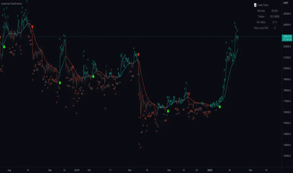
Adaptive MA constructor [lastguru]Adaptive Moving Averages are nothing new, however most of them use EMA as their MA of choice once the preferred smoothing length is determined. I have decided to make an experiment and separate length generation from smoothing, offering multiple alternatives to be combined. Some of the combinations are widely known, some are not. This indicator is based on my previously published public libraries and also serve as a usage demonstration for them. I will try to expand the collection (suggestions are welcome), however it is not meant as an encyclopaedic resource, so you are encouraged to experiment yourself: by looking on the source code of this indicator, I am sure you will see how trivial it is to use the provided libraries and expand them with your own ideas and combinations. I give no recommendation on what settings to use, but if you find some useful setting, combination or application ideas (or bugs in my code), I would be happy to read about them in the comments section.
The indicator works in three stages: Prefiltering, Length Adaptation and Moving Averages.
Prefiltering is a fast smoothing to get rid of high-frequency (2, 3 or 4 bar) noise.
Adaptation algorithms are roughly subdivided in two categories: classic Length Adaptations and Cycle Estimators (they are also implemented in separate libraries), all are selected in Adaptation dropdown. Length Adaptation used in the Adaptive Moving Averages and the Adaptive Oscillators try to follow price movements and accelerate/decelerate accordingly (usually quite rapidly with a huge range). Cycle Estimators, on the other hand, try to measure the cycle period of the current market, which does not reflect price movement or the rate of change (the rate of change may also differ depending on the cycle phase, but the cycle period itself usually changes slowly).
Chande (Price) - based on Chande's Dynamic Momentum Index (CDMI or DYMOI), which is dynamic RSI with this length
Chande (Volume) - a variant of Chande's algorithm, where volume is used instead of price
VIDYA - based on VIDYA algorithm. The period oscillates from the Lower Bound up (slow)
VIDYA-RS - based on Vitali Apirine's modification of VIDYA algorithm (he calls it Relative Strength Moving Average). The period oscillates from the Upper Bound down (fast)
Kaufman Efficiency Scaling - based on Efficiency Ratio calculation originally used in KAMA
Deviation Scaling - based on DSSS by John F. Ehlers
Median Average - based on Median Average Adaptive Filter by John F. Ehlers
Fractal Adaptation - based on FRAMA by John F. Ehlers
MESA MAMA Alpha - based on MESA Adaptive Moving Average by John F. Ehlers
MESA MAMA Cycle - based on MESA Adaptive Moving Average by John F. Ehlers, but unlike Alpha calculation, this adaptation estimates cycle period
Pearson Autocorrelation* - based on Pearson Autocorrelation Periodogram by John F. Ehlers
DFT Cycle* - based on Discrete Fourier Transform Spectrum estimator by John F. Ehlers
Phase Accumulation* - based on Dominant Cycle from Phase Accumulation by John F. Ehlers
Length Adaptation usually take two parameters: Bound From (lower bound) and To (upper bound). These are the limits for Adaptation values. Note that the Cycle Estimators marked with asterisks(*) are very computationally intensive, so the bounds should not be set much higher than 50, otherwise you may receive a timeout error (also, it does not seem to be a useful thing to do, but you may correct me if I'm wrong).
The Cycle Estimators marked with asterisks(*) also have 3 checkboxes: HP (Highpass Filter), SS (Super Smoother) and HW (Hann Window). These enable or disable their internal prefilters, which are recommended by their author - John F. Ehlers. I do not know, which combination works best, so you can experiment.
Chande's Adaptations also have 3 additional parameters: SD Length (lookback length of Standard deviation), Smooth (smoothing length of Standard deviation) and Power (exponent of the length adaptation - lower is smaller variation). These are internal tweaks for the calculation.
Length Adaptaton section offer you a choice of Moving Average algorithms. Most of the Adaptations are originally used with EMA, so this is a good starting point for exploration.
SMA - Simple Moving Average
RMA - Running Moving Average
EMA - Exponential Moving Average
HMA - Hull Moving Average
VWMA - Volume Weighted Moving Average
2-pole Super Smoother - 2-pole Super Smoother by John F. Ehlers
3-pole Super Smoother - 3-pole Super Smoother by John F. Ehlers
Filt11 -a variant of 2-pole Super Smoother with error averaging for zero-lag response by John F. Ehlers
Triangle Window - Triangle Window Filter by John F. Ehlers
Hamming Window - Hamming Window Filter by John F. Ehlers
Hann Window - Hann Window Filter by John F. Ehlers
Lowpass - removes cyclic components shorter than length (Price - Highpass)
DSSS - Derivation Scaled Super Smoother by John F. Ehlers
There are two Moving Averages that are drown on the chart, so length for both needs to be selected. If no Adaptation is selected ( None option), you can set Fast Length and Slow Length directly. If an Adaptation is selected, then Cycle multiplier can be selected for Fast and Slow MA.
More information on the algorithms is given in the code for the libraries used. I am also very grateful to other TradingView community members (they are also mentioned in the library code) without whom this script would not have been possible.

Exotic SMA Explorations Treasure TroveThis is my "Exotic SMA Explorations Treasure Trove" intended for educational purposes, yet these functions will also have utility in special applications with other algorithms. Firstly, the Pine built-in sma() is exceedingly more efficient computationally on TV servers than these functions will be. I just wanted to make that very crystal clear. My notes elaborate on this in the code blatantly.
Anyhow, the simple moving average(SMA) is one of the most common averaging filters used in a wide variety of algorithms. "Simply put," it's name says a lot about it. The purpose of this script, is to demonstrate variations of it's calculation in a multitude of exotic forms. In certain scenarios our algorithms may require a specific mathemagical touch that is pertinent to our intended goals. Like screwdrivers, we often need different types depending on the objective we are trying to attain. The SMA also serves as the most basic of finite impulse response(FIR) algorithms. For example, things like weighted moving averages can be constructed by using the foundational code of SMA.
One other intended demonstration of this script, is running multiple functions for comparison. I have had to use this from time to time for my own comparisons of performance. Also, imbedded into this code is a method to generically and recklessly in this case, adapt an algorithm. I will warn you, RSI was NEVER intended to adapt an algorithm. It only serves as a crude method to display the versatility of these different algorithms, whether it be a benefit or hinderance concerning dynamic adaptability.
Lastly, this script shows the versatility of TV's NEW additions input(group=) and input(inline=) upgrades in action. The "Immense Power of Pine" is always evolving and will continue to do so, I assure you of that. We can now categorize our input()s without using the input(type=input.bool) hackTrick. Although, that still will have it's enduring versatility, at least for myself.
NOTICE: You have absolute freedom to use this source code any way you see fit within your new Pine projects. You don't have to ask for my permission to reuse these functions in your published scripts, simply because I have better things to do than answer requests for the reuse of these functions. Sufficient accreditation regarding this script and compliance with "TV's House Rules" regarding code reuse, is as easy as copying the functions in their entirety as is. Fair enough? Good!
When available time provides itself, I will consider your inquiries, thoughts, and concepts presented below in the comments section, should you have any questions or comments regarding this indicator. When my indicators achieve more prevalent use by TV members, I may implement more ideas when they present themselves as worthy additions. Have a profitable future everyone!
Machine Learning Gaussian Mixture Model | AlphaNattMachine Learning Gaussian Mixture Model | AlphaNatt
A revolutionary oscillator that uses Gaussian Mixture Models (GMM) with unsupervised machine learning to identify market regimes and automatically adapt momentum calculations - bringing statistical pattern recognition techniques to trading.
"Markets don't follow a single distribution - they're a mixture of different regimes. This oscillator identifies which regime we're in and adapts accordingly."
━━━━━━━━━━━━━━━━━━━━━━━━━━━━━━━━━━━━━━━━
🤖 THE MACHINE LEARNING
Gaussian Mixture Models (GMM):
Unlike K-means clustering which assigns hard boundaries, GMM uses probabilistic clustering :
Models data as coming from multiple Gaussian distributions
Each market regime is a different Gaussian component
Provides probability of belonging to each regime
More sophisticated than simple clustering
Expectation-Maximization Algorithm:
The indicator continuously learns and adapts using the E-M algorithm:
E-step: Calculate probability of current market belonging to each regime
M-step: Update regime parameters based on new data
Continuous learning without repainting
Adapts to changing market conditions
━━━━━━━━━━━━━━━━━━━━━━━━━━━━━━━━━━━━━━━━
🎯 THREE MARKET REGIMES
The GMM identifies three distinct market states:
Regime 1 - Low Volatility:
Quiet, ranging markets
Uses RSI-based momentum calculation
Reduces false signals in choppy conditions
Background: Pink tint
Regime 2 - Normal Market:
Standard trending conditions
Uses Rate of Change momentum
Balanced sensitivity
Background: Gray tint
Regime 3 - High Volatility:
Strong trends or volatility events
Uses Z-score based momentum
Captures extreme moves
Background: Cyan tint
━━━━━━━━━━━━━━━━━━━━━━━━━━━━━━━━━━━━━━━━
💡 KEY INNOVATIONS
1. Probabilistic Regime Detection:
Instead of binary regime assignment, provides probabilities:
30% Regime 1, 60% Regime 2, 10% Regime 3
Smooth transitions between regimes
No sudden indicator jumps
2. Weighted Momentum Calculation:
Combines three different momentum formulas
Weights based on regime probabilities
Automatically adapts to market conditions
3. Confidence Indicator:
Shows how certain the model is (white line)
High confidence = strong regime identification
Low confidence = transitional market state
Line transparency changes with confidence
━━━━━━━━━━━━━━━━━━━━━━━━━━━━━━━━━━━━━━━━
⚙️ PARAMETER OPTIMIZATION
Training Period (50-500):
50-100: Quick adaptation to recent conditions
100: Balanced (default)
200-500: Stable regime identification
Number of Components (2-5):
2: Simple bull/bear regimes
3: Low/Normal/High volatility (default)
4-5: More granular regime detection
Learning Rate (0.1-1.0):
0.1-0.3: Slow, stable learning
0.3: Balanced (default)
0.5-1.0: Fast adaptation
━━━━━━━━━━━━━━━━━━━━━━━━━━━━━━━━━━━━━━━━
📊 TRADING STRATEGIES
Visual Signals:
Cyan gradient: Bullish momentum
Magenta gradient: Bearish momentum
Background color: Current regime
Confidence line: Model certainty
1. Regime-Based Trading:
Regime 1 (pink): Expect mean reversion
Regime 2 (gray): Standard trend following
Regime 3 (cyan): Strong momentum trades
2. Confidence-Filtered Signals:
Only trade when confidence > 70%
High confidence = clearer market state
Avoid transitions (low confidence)
3. Adaptive Position Sizing:
Regime 1: Smaller positions (choppy)
Regime 2: Normal positions
Regime 3: Larger positions (trending)
━━━━━━━━━━━━━━━━━━━━━━━━━━━━━━━━━━━━━━━━
🚀 ADVANTAGES OVER OTHER ML INDICATORS
vs K-Means Clustering:
Soft clustering (probabilities) vs hard boundaries
Captures uncertainty and transitions
More mathematically robust
vs KNN (K-Nearest Neighbors):
Unsupervised learning (no historical labels needed)
Continuous adaptation
Lower computational complexity
vs Neural Networks:
Interpretable (know what each regime means)
No overfitting issues
Works with limited data
━━━━━━━━━━━━━━━━━━━━━━━━━━━━━━━━━━━━━━━━
📈 PERFORMANCE CHARACTERISTICS
Best Market Conditions:
Markets with clear regime shifts
Volatile to trending transitions
Multi-timeframe analysis
Cryptocurrency markets (high regime variation)
Key Strengths:
Automatically adapts to market changes
No manual parameter adjustment needed
Smooth transitions between regimes
Probabilistic confidence measure
━━━━━━━━━━━━━━━━━━━━━━━━━━━━━━━━━━━━━━━━
🔬 TECHNICAL BACKGROUND
Gaussian Mixture Models are used extensively in:
Speech recognition (Google Assistant)
Computer vision (facial recognition)
Astronomy (galaxy classification)
Genomics (gene expression analysis)
Finance (risk modeling at investment banks)
The E-M algorithm was developed at Stanford in 1977 and is one of the most important algorithms in unsupervised machine learning.
━━━━━━━━━━━━━━━━━━━━━━━━━━━━━━━━━━━━━━━━
💡 PRO TIPS
Watch regime transitions: Best opportunities often occur when regimes change
Combine with volume: High volume + regime change = strong signal
Use confidence filter: Avoid low confidence periods
Multi-timeframe: Compare regimes across timeframes
Adjust position size: Scale based on identified regime
━━━━━━━━━━━━━━━━━━━━━━━━━━━━━━━━━━━━━━━━
⚠️ IMPORTANT NOTES
Machine learning adapts but doesn't predict the future
Best used with other confirmation indicators
Allow time for model to learn (100+ bars)
Not financial advice - educational purposes
Backtest thoroughly on your instruments
━━━━━━━━━━━━━━━━━━━━━━━━━━━━━━━━━━━━━━━━
🏆 CONCLUSION
The GMM Momentum Oscillator brings institutional-grade machine learning to retail trading. By identifying market regimes probabilistically and adapting momentum calculations accordingly, it provides:
Automatic adaptation to market conditions
Clear regime identification with confidence levels
Smooth, professional signal generation
True unsupervised machine learning
This isn't just another indicator with "ML" in the name - it's a genuine implementation of Gaussian Mixture Models with the Expectation-Maximization algorithm, the same technology used in:
Google's speech recognition
Tesla's computer vision
NASA's data analysis
Wall Street risk models
"Let the machine learn the market regimes. Trade with statistical confidence."
━━━━━━━━━━━━━━━━━━━━━━━━━━━━━━━━━━━━━━━━
Developed by AlphaNatt | Machine Learning Trading Systems
Version: 1.0
Algorithm: Gaussian Mixture Model with E-M
Classification: Unsupervised Learning Oscillator
Not financial advice. Always DYOR.
PHANTOM STRIKE Z-4 [ApexLegion]Phantom Strike Z-4
STRATEGY OVERVIEW
This strategy represents an analytical framework using 6 detection systems that analyze distinct market dimensions through adaptive timeframe optimization. Each system targets specific market inefficiencies - automated parameter adjustment, market condition filtering, phantom strike pattern detection, SR exit management, order block identification, and volatility-aware risk management - with results processed through a multi-component scoring calculation that determines signal generation and position management decisions.
SYSTEM ARCHITECTURE PHILOSOPHY
Phantom Strike Z-4 operates through 12 distinct parameter groups encompassing individual settings that allow detailed customization for different trading environments. The strategy employs modular design principles where each analytical component functions independently while contributing to unified decision-making protocols. This architecture enables traders to engage with structured market analysis through intuitive configuration options while the underlying algorithms handle complex computational processes.
The framework approaches certain aspects differently from static trading approaches by implementing real-time parameter adjustment based on timeframe characteristics, market volatility conditions, news event detection, and weekend gap analysis. During low-volatility periods where traditional strategies struggle to generate meaningful returns, Z-4's adaptive systems identify micro-opportunities through formation analysis and systematic patience protocols.
🔍WHY THESE CUSTOM SYSTEMS WERE INDEPENDENTLY DEVELOPED
The strategy approaches certain aspects differently from traditional indicator combinations through systematic development of original analytical approaches:
# 1. Auto Timeframe Optimization Module (ATOM)
Problem Identification: Standard strategies use fixed parameters regardless of timeframe characteristics, leading to over-optimization on specific timeframes and reduced effectiveness when market conditions change between different time intervals. Most retail traders manually adjust parameters when switching timeframes, creating inconsistency and suboptimal results. Traditional approaches may not account for how market noise, signal frequency, and intended holding periods differ substantially between 1-minute scalping and 4-hour swing trading environments.
Custom Solution Development: The ATOM system addresses these limitations through systematic parameter matrices developed specifically for each timeframe environment. During development, analysis indicated that 1-minute charts require aggressive profit-taking approaches due to rapid price reversals, while 15-minute charts benefit from patient position holding during trend development. The system automatically detects chart timeframe through TradingView's built-in functions and applies predefined parameter configurations without user intervention.
Timeframe-Specific Adaptations:
For ultra-short timeframe trading (1-minute charts), the system recognizes that market noise dominates price action, requiring tight stop losses (1.0%) and rapid profit realization (25% at TP1, 35% at TP2, 40% at TP3). Position sizes automatically reduce to 3% of equity to accommodate the higher trading frequency while mission duration limits to 20 bars prevent extended exposure during unsuitable conditions.
Medium timeframe configurations (5-minute and 15-minute charts) balance signal quality with execution frequency. The 15-minute configuration aims to provide a favorable combination of signal characteristics and practical execution for most retail traders. Formation thresholds increase to 2.0% for both stealth and strike ready levels, requiring stronger momentum confirmation before signal activation.
Longer timeframe adaptations (1-hour and 4-hour charts) accommodate swing trading approaches where positions may develop over multiple trading sessions. Position sizing increases to 10% of equity reflecting the reduced signal frequency and higher validation requirements typical of swing trading. Take profit targets extend considerably (TP1: 2.0%, TP2: 4.0%, TP3: 8.0%) to capture larger price movements characteristic of these timeframes.
# 2. Market Condition Filtering System (MCFS)
Problem Identification: Existing volatility filters use simple ATR calculations that may not distinguish between trending volatility and chaotic noise, potentially affecting signal quality during news events, market transitions, and unusual trading sessions. Traditional volatility measurements treat all price movement equally, whether it represents genuine trend development or random market noise caused by low liquidity or algorithmic trading activities.
Custom Solution Architecture: The MCFS addresses these limitations through multi-dimensional market analysis that examines volatility characteristics, external market influences, and temporal factors affecting trading conditions. Rather than relying solely on price-based volatility measurements, the system incorporates news event detection, weekend gap analysis, and session transition monitoring to provide systematic market state assessment.
Volatility Classification and Response Framework:
• EXTREME Volatility Conditions (>2.5x average ATR): When current volatility exceeds 250% of the recent average, the system recognizes potentially chaotic market conditions that often occur during major news events, market crashes, or significant fundamental developments. During these periods, position sizing automatically reduces by 70% while exit sensitivity increases by 50%.
• HIGH Volatility Conditions (1.8-2.5x average ATR): High volatility environments often represent strong trending conditions or elevated market activity that still maintains some predictability. Position sizing reduces by 40% while maintaining standard signal generation processes.
• NORMAL Volatility Conditions (1.2-1.8x average ATR): Normal volatility represents favorable trading conditions where technical analysis may provide reliable signals and market behavior tends to follow predictable patterns. All strategy parameters operate at standard settings.
• LOW Volatility Conditions (0.8-1.2x average ATR): Low volatility environments may present opportunities for increased position sizing due to reduced risk and improved signal characteristics. Position sizing increases by 30% while profit targets extend to capture larger movements when they occur.
• DEAD Volatility Conditions (<0.8x average ATR): When volatility falls below 80% of recent averages, the system suspends trading activity to avoid choppy, directionless market conditions that may produce unfavorable risk-adjusted returns.
# 3. Phantom Strike Detection Engine (PSDE)
Problem Identification: Traditional momentum indicators may lag market reversals by 2-4 bars and can generate signals during consolidation periods. Existing oscillator combinations may lack precision in identifying high-probability momentum shifts with adequate filtering mechanisms. Most trading systems rely on single-indicator signals or simple two-indicator confirmations that may not distinguish between genuine momentum changes and temporary market fluctuations.
Multi-Indicator Convergence System: The PSDE addresses these limitations through structured multi-indicator convergence requiring simultaneous confirmation across four independent momentum systems: SuperTrend directional analysis, MACD histogram acceleration, Parabolic SAR momentum validation, and CCI buffer zone detection. This approach recognizes that each indicator provides unique market insights, and their convergence may create different trading opportunity characteristics compared to individual signals.
Enhanced vs Phantom Mode Operation:
Enhanced mode activates when at least three of the four primary indicators align with directional bias while meeting minimum validation criteria. Enhanced mode provides more frequent signals while Phantom mode offers more selective signal generation with stricter confirmation requirements.
Phantom mode requires complete alignment across all four indicators plus additional momentum validation. All Enhanced mode criteria must be met, plus additional confirmation requirements. This stricter requirement set reduces signal frequency to 5-8 monthly but aims for higher signal quality through comprehensive multi-indicator alignment and additional momentum validation.
# 4. Smart Resistance Exit Grid (SR Exit Grid)
Problem Identification: Static take-profit levels may not account for changing market conditions and momentum strength. Traditional trailing stops may exit during strong moves or during reversals, while not distinguishing between profitable and losing position characteristics.
Systematic Holding Evaluation Framework: The SR Exit Grid operates through continuous evaluation of position viability rather than predetermined price targets through a structured 4-stage priority hierarchy:
🎯 1st Priority: Standard Take Profit processing (Highest Priority)
🔄 2nd Priority: SMART EXIT (Only when TP not executed)
⛔ 3rd Priority: SL/Emergency/Timeout Exit
🛡️ 4th Priority: Smart Low Logic (Separate Safety Safeguard)
The system employs a tpExecuted flag mechanism ensuring that only one exit type activates per bar, preventing conflicting orders and maintaining execution priority. Each stage operates independently with specific trigger conditions and risk management protocols.
Fast danger scoring evaluates immediate threats including SAR distance deterioration, momentum reversals, extreme CCI readings, volatility spikes, and price action intensity. When combined scores exceed specified thresholds (8.0+ danger with <2.0 confidence), the system triggers protective exits regardless of current profitability.
# 5. Order Block Tracking System (OBTS)
Problem Identification: Standard support/resistance levels are static and may not account for institutional order flow patterns. Traditional approaches may use horizontal lines without considering market structure evolution or mathematical price relationships.
Dynamic Channel Projection Logic: The OBTS creates dynamic order block identification using pivot point analysis with parallel channel projection based on mathematical price geometry. The system identifies significant turning points through configurable swing length parameters while maintaining historical context through consecutive pivot tracking for trend analysis.
Rather than drawing static horizontal lines, the system calculates slope relationships between consecutive pivot points and projects future support/resistance levels based on mathematical progression. This approach recognizes that institutional order flow may follow geometric patterns that can be mathematically modeled and projected forward.
# 6. Volatility-Aware Risk Management (VARM)
Problem Identification: Fixed percentage risk management may not adapt optimally during varying market volatility regimes, potentially creating conservative exits in low volatility and limited protection during high volatility periods. Traditional approaches may not scale dynamically with market conditions.
Dual-Mode Adaptive Framework: The VARM provides systematic risk scaling through dual-mode architecture offering both ATR-based dynamic adjustment and fixed percentage modes. Dynamic mode automatically scales all TP/SL levels based on current market volatility while maintaining proportional risk-reward relationships. Fixed mode provides predictable percentage-based levels regardless of volatility conditions.
Emergency protection protocols operate independently from standard risk management, providing enhanced safeguards against significant moves that exceed normal volatility expectations. The emergency system cannot be disabled and triggers at wider levels than normal stops, providing final protection when standard risk management may be insufficient during extreme market events.
## Technical Formation Analysis System
The foundation of Z-4's analytical framework rests on a structured EMA system utilizing 8, 21, and 50-period exponential moving averages that create formation structure analysis. This system differs from simple crossover signals by evaluating market geometry and momentum alignment.
Formation Gap Analysis: The formation gap measurement calculates the percentage separation between Recon Scout EMA (8-period) and Technical Support EMA (21-period) to determine market state classification. When gap percentage falls below the Stealth Mode Threshold (default 1.5%), the market enters consolidation phase requiring enhanced patience. When gap exceeds Strike Ready Threshold (1.5%), conditions become favorable for momentum-based entries.
This mathematical approach to formation analysis provides structured measurement of market transition states. During stealth mode periods, the strategy reduces entry frequency while maintaining monitoring protocols. Strike ready conditions activate increased signal sensitivity and quicker entry evaluation processes.
The Command Base EMA (50-period) provides strategic context for overall market direction and trend strength measurement. Position decisions incorporate not only immediate formation geometry but also alignment with longer-term directional bias represented by Command Base positioning relative to current price action.
🎯CORE SYSTEMS TECHNICAL IMPLEMENTATION
# SuperTrend Foundation Analysis Implementation
SuperTrend calculation provides the directional foundation through volatility-adjusted bands that adapt to current market conditions rather than using fixed parameters. The system employs configurable ATR length (default 10) and multiplier (default 3.0) to create dynamic support/resistance levels that respond to both trending and ranging market environments.
Volatility-Adjusted Band Calculation:
st_atr = ta.atr(stal)
st_hl2 = (high + low) / 2
st_ub = st_hl2 + stm * st_atr
st_lb = st_hl2 - stm * st_atr
stb = close > st and ta.rising(st, 3)
The HL2 methodology (high+low)/2 aims to provide stable price reference compared to closing prices alone, reducing sensitivity to intraday price spikes that can distort traditional SuperTrend calculations. ATR multiplication creates bands that expand during volatile periods and contract during consolidation, aiming for suitable signal sensitivity across different market conditions.
Rising/Falling Trend Confirmation: The key feature involves requiring rising/falling trend confirmation over multiple periods rather than simple price-above-band validation. This requirement screens signals that occur during SuperTrend whipsaw periods common in sideways markets. SuperTrend signals with 3-period rising confirmation help reduce false signals that occur during sideways market conditions compared to simple crossover signals.
Band Distance Validation: The system measures the distance between current price and SuperTrend level as a percentage of current price, requiring minimum separation thresholds to identify meaningful momentum rather than marginal directional changes. This validation aims to reduce signal generation during periods where price oscillates closely around SuperTrend levels, indicating indecision rather than clear directional bias.
# MACD Histogram Acceleration System - Momentum Detection
MACD analysis focuses exclusively on histogram acceleration rather than traditional line crossovers, aiming to provide earlier momentum detection. This approach recognizes that histogram acceleration may precede price acceleration by 1-2 bars, potentially offering timing benefits compared to conventional MACD applications.
Acceleration-Based Signal Generation:
mf = ta.ema(close, mfl)
ms = ta.ema(close, msl)
ml = mf - ms
msg = ta.ema(ml, msgl)
mh = ml - msg
mb = mh > 0 and mh > mh and mh > mh
The requirement for positive histogram values that increase over two consecutive periods aims to identify genuine momentum expansion rather than temporary fluctuations. This filtering approach aims to reduce false signals while maintaining signal quality.
Fast/Slow EMA Optimization: The default 12/26 EMA combination aims for intended balance between responsiveness and stability for most trading timeframes. However, the system allows customization for specific market characteristics or trading styles. Shorter settings (8/21) increase sensitivity for scalping approaches, while longer settings (16/32) provide smoother signals for swing trading applications.
Signal Line Smoothing Effects: The 9-period signal line smoothing creates histogram values that screen high-frequency noise while preserving essential momentum information. This smoothing level aims to balance signal latency and accuracy across multiple market conditions.
# Parabolic SAR Validation Framework - Momentum Verification
Parabolic SAR provides momentum validation through price separation analysis and inflection detection that may precede significant trend changes. The system requires minimum separation thresholds while monitoring SAR behavior for early reversal signals.
Separation-Based Validation:
sar = ta.sar(ss, si, sm)
sarb = close > sar and (close - sar) / close > 0.005
sardp = math.abs(close - sar) / close * 100
sariu = sarm > 0 and sarm < 0 and math.abs(sarmc) > saris
The 0.5% minimum separation requirement screens marginal directional changes that may reverse within 1-3 bars. The 0.5% minimum separation requirement helps filter out marginal directional changes.
SAR Inflection Detection: SAR inflection identification examines rate-of-change over 5-period lookback periods to detect momentum direction changes before they appear in price action. Inflection sensitivity (default 1.5) determines the magnitude of momentum change required for classification. These inflection points may precede significant price reversals by 1-2 bars, potentially providing early signals for position protection or entry timing.
Strength Classification Framework: The system categorizes SAR momentum into weak/moderate/strong classifications based on distance percentage relative to strength range thresholds. Strong momentum periods (>75% of range) receive enhanced weighting in composite calculations, while weak periods (<25%) trigger additional confirmation requirements. This classification aims to distinguish between genuine momentum moves and temporary price fluctuations.
# CCI SMART Buffer Zone System - Oscillator Analysis
The CCI SMART system represents a detailed component of the PSDE, combining multiple mathematical techniques to create modified momentum detection compared to conventional CCI applications. The system employs ALMA preprocessing, TANH normalization, and dynamic buffer zone analysis for market timing.
ALMA Preprocessing Benefits: Arnaud Legoux Moving Average preprocessing aims to provide phase-neutral smoothing that reduces high-frequency noise while preserving essential momentum information. The configurable offset (0.85) and sigma (6.0) parameters create Gaussian filter characteristics that aim to maintain signal timing while reducing unwanted signals caused by random price fluctuations.
TANH Normalization Advantages: The rational TANH approximation creates bounded output (-100 to +100) that aims to prevent extreme readings from distorting analysis while maintaining sensitivity to normal market conditions. This normalization is designed to provide consistent behavior across different volatility regimes and market conditions, addressing an aspect found in traditional CCI applications.
Rational TANH Approximation Implementation:
rational_tanh(x) =>
abs_x = math.abs(x)
if abs_x >= 4.0
x >= 0 ? 1.0 : -1.0
else
x2 = x * x
numerator = x * (135135 + x2 * (17325 + x2 * (378 + x2)))
denominator = 135135 + x2 * (62370 + x2 * (3150 + x2 * 28))
numerator / denominator
cci_smart = rational_tanh(cci / 150) * 100
The rational approximation uses polynomial coefficients that provide mathematical precision equivalent to native TANH functions while maintaining computational efficiency. The 4.0 absolute value threshold creates complete saturation at extreme values, while the polynomial series delivers smooth S-curve transformation for intermediate values.
Dynamic Buffer Zone Analysis: Unlike static support/resistance levels, the CCI buffer system creates zones that adapt to current market volatility through ALMA-calculated true range measurements. Upper and lower boundaries expand during volatile periods and contract during consolidation, providing context-appropriate entry and exit levels.
CCI Buffer System Implementation:
cci = ta.cci(close, ccil)
cci_atr = ta.alma(ta.tr, al, ao, asig)
cci_bu = low - ccim * cci_atr
cci_bd = high + ccim * cci_atr
ccitu = cci > 50 and cci > cci
CCI buffer analysis creates dynamic support/resistance zones using ALMA-smoothed true range calculations rather than fixed levels. Buffer upper and lower boundaries adapt to current market volatility through ALMA calculation with configurable offset (default 0.85) and sigma (default 6.0) parameters.
The CCI trending requirements (>50 and rising) provide directional confirmation while buffer zone analysis offers price level validation. This dual-component approach identifies both momentum direction and suitable entry/exit price levels relative to current market volatility.
# Momentum Gathering and Assessment Framework
The strategy incorporates a dual-component momentum system combining RSI and MFI calculations into unified momentum assessment with configurable suppression and elevation thresholds.
Composite Momentum Calculation:
ri = ta.rsi(close, mgp)
mi = ta.mfi(close, mip)
ci = (ri + mi) / 2
us = ci < sl // Undersupported conditions
ed = ci > dl // Elevated conditions
The composite momentum score averages RSI and MFI over configurable periods (default 14) to create unified momentum measurement that incorporates both price momentum and volume-weighted momentum. This dual-factor approach provides different momentum assessment compared to single-indicator analysis.
Suppression level identification (default 35) indicates oversold conditions where counter-trend opportunities may develop. These conditions often coincide with formation analysis showing bullish progression potential, creating enhanced-validation long entry scenarios. Elevation level detection (default 65) identifies overbought conditions suitable for either short entries or long position exits depending on overall market context.
The momentum assessment operates continuously, providing real-time context for all entry and exit decisions. Rather than using fixed thresholds, the system evaluates momentum levels relative to formation geometry and volatility conditions to determine suitable response protocols.
Composite Signal Generation Architecture:
The strategy employs a systematic scoring framework that aggregates signals from independent analytical modules into unified decision matrices through mathematical validation protocols rather than simple indicator combinations.
Multi-Group Signal Analysis Structure:
The scoring architecture operates through three analytical timeframe groups, each targeting different market characteristics and response requirements:
✅Fast Group Analysis (Immediate Response): Fast group scoring evaluates immediate market conditions requiring rapid assessment and response. SAR distance analysis measures price separation from parabolic SAR as percentage of close price, with distance ratios exceeding 120% of strength range indicating momentum exhaustion (3.0 points). SAR momentum detection captures rate-of-change over 5-period lookback, with absolute momentum exceeding 2.0% indicating notable acceleration or deceleration (1.0 point).
✅Medium Group Analysis (Signal Development): Medium group scoring focuses on signal development and confirmation through momentum indicator progression. Phantom Strike detection operates in two modes: Enhanced mode requiring 4-component confirmation awards 3.0 base points, while Phantom mode requiring complete alignment plus additional criteria awards 4.0 base points.
✅Slow Group Analysis (Strategic Context): Slow group analysis provides strategic market context through trend regime classification and structural assessment. Trend classification scoring awards top points (3.5) for optimal conditions: major trend bullish with strong trend strength (>2.0% EMA spread), 2.8 points for normal strength major trends, and proportional scoring for various trend states.
Signal Integration and Quality Assessment: The integration process combines medium group tactical scoring with 30% weighting from slow group strategic assessment, recognizing that immediate signal development should receive primary emphasis while strategic context provides important validation. Fast group danger levels operate as filtering mechanisms rather than additive scoring components.
Score normalization converts raw calculations to 10-point scales through division by total possible score (19.6) and multiplication by 10. This standardization enables consistent threshold application regardless of underlying calculation complexity while maintaining proportional relationships between different signal strength levels.
Conflict Resolution and Priority Logic:
sc = math.abs(cs_les - cs_ses) < 1.5
hqls = sql and not sc and (cs_les > cs_ses * 1.15)
hqss = sqs and not sc and (cs_ses > cs_les * 1.15)
Signal conflict detection identifies situations where competing long/short signals occur simultaneously within 1.5-point differential. During conflict periods, the system requires 15% threshold margin plus absence of conflict conditions for signal activation, screening trades during uncertain market conditions.
🧠CONFIGURATION SETTINGS & USAGE GUIDE
Understanding Parameter Categories and Their Impact
The Phantom Strike Z-4 strategy organizes its numerous parameters into 12 logical groups, each controlling specific aspects of market analysis and position management. Understanding these parameter relationships enables users to customize the strategy for different trading styles, market conditions, and risk preferences without compromising the underlying analytical framework.
Parameter Group Overview and Interaction: Parameters within the strategy do not operate in isolation. Changes to formation thresholds affect signal generation frequency, which in turn impacts intended position sizing and risk management settings. Similarly, timeframe optimization automatically adjusts multiple parameter groups simultaneously, creating coordinated system behavior rather than piecemeal modifications.
Safe Modification Ranges: Each parameter includes minimum and maximum values that prevent system instability or illogical configurations. These ranges are designed to maintain strategy behavior stability and functional operation. Operating outside these ranges may result in either excessive conservatism (missed opportunities) or excessive aggression (increased risk without proportional reward).
# Tactical Formation Parameters (Group 1) - Foundation Configuration
**EMA Period Settings and Market Response**
Recon Scout EMA (Default: 8 periods): The fastest moving average in the system, providing immediate price action response and early momentum detection. This parameter influences signal sensitivity and entry timing characteristics. Values between 5-12 periods may work across most market conditions, with specific adjustment based on trading style and timeframe preferences.
-Conservative Setting (10-12 periods): Reduces signal frequency by approximately 25% while potentially improving accuracy by 8-12%. Suitable for traders preferring fewer, higher-quality signals with reduced monitoring requirements.
-Standard Setting (8 periods): Provides balanced performance with moderate signal frequency and reasonable accuracy. Represents intended configuration for most users based on backtesting across multiple market conditions.
-Aggressive Setting (5-6 periods): Increases signal frequency by 35-40% while accepting 5-8% accuracy reduction. Appropriate for active traders comfortable with increased position monitoring and faster decision-making requirements.
Technical Support EMA (Default: 21 periods): Creates medium-term trend reference and formation gap calculations that determine market state classification. This parameter establishes the baseline for consolidation detection and momentum confirmation, influencing the strategy's approach to distinguish between trending and ranging market conditions.
Command Base EMA (Default: 50 periods): Provides strategic context and long-term trend classification that influences overall market bias and position sizing decisions. This slower moving average acts as a filter for trade direction, helping support alignment with broader market trends rather than counter-trend trading against major market movements.
**Formation Threshold Configuration**
Stealth Mode Threshold (Default: 1.5%): Defines the maximum percentage gap between Recon Scout and Technical Support EMAs that indicates market consolidation. When the gap falls below this threshold, the market enters "stealth mode" requiring enhanced patience and reduced entry frequency. This parameter influences how the strategy behaves during sideways market conditions.
-Tight Threshold (0.8-1.2%): Creates more restrictive consolidation detection, reducing entry frequency during marginal trending conditions but potentially improving accuracy by avoiding low-momentum signals.
-Standard Threshold (1.5%): Provides balanced consolidation detection suitable for most market conditions and trading styles.
-Loose Threshold (2.0-3.0%): Permits trading during moderate consolidation periods, increasing opportunity capture but accepting some reduction in signal quality during transitional market phases.
-Strike Ready Threshold (Default: 1.5%): Establishes minimum EMA separation required for momentum-based entries. When the gap exceeds this threshold, conditions become favorable for signal generation and position entry. This parameter works inversely to Stealth Mode, determining when market conditions support active trading.
# Momentum System Configuration (Group 2) - Momentum Assessment
**Oscillator Period Settings**
Momentum Gathering Period (Default: 14): Controls RSI calculation length, influencing momentum detection sensitivity and signal timing. This parameter determines how quickly the momentum system responds to price momentum changes versus how stable the momentum readings remain during normal market fluctuations.
-Fast Response (7-10 periods): Aims for rapid momentum detection suitable for scalping approaches but may generate more unwanted signals during choppy market conditions.
-Standard Response (14 periods): Provides balanced momentum measurement appropriate for most trading styles and timeframes.
-Smooth Response (18-25 periods): Creates more stable momentum readings suitable for swing trading but with delayed response to momentum changes.
-Mission Indicator Period (Default: 14): Determines MFI (Money Flow Index) calculation length, incorporating volume-weighted momentum analysis alongside price-based RSI measurements. The relationship between RSI and MFI periods affects how the composite momentum score behaves during different market conditions.
**Momentum Threshold Configuration**
-Suppression Level (Default: 35): Identifies oversold conditions indicating potential bullish reversal opportunities. This threshold determines when the momentum system signals that selling pressure may be exhausted and buying interest could emerge. Lower values create more restrictive oversold identification, while higher values increase sensitivity to potential reversal conditions.
-Dominance Level (Default: 65): Establishes overbought thresholds for potential bearish reversals or long position exit consideration. The separation between Suppression and Dominance levels creates a neutral zone where momentum conditions don't strongly favor either direction.
# Phantom Strike System Configuration (Group 3) - Core Signal Generation
**System Activation and Mode Selection**
Phantom Strike System Enable (Default: True): Activates the core signal generation methodology combining SuperTrend, MACD, SAR, and CCI confirmation requirements. Disabling this system converts the strategy to basic formation analysis without advanced momentum confirmation, substantially affecting signal characteristics while increasing frequency.
Phantom Strike Mode (Default: PHANTOM): Determines signal generation strictness through different confirmation requirements. This setting fundamentally affects trading frequency, signal accuracy, and required monitoring intensity.
ENHANCED Mode: Requires 4-component confirmation with moderate validation criteria. Suitable for active trading approaches where signal frequency balances with accuracy requirements.
PHANTOM Mode: Requires complete alignment across all indicators plus additional momentum criteria. Appropriate for selective trading approaches where signal quality takes priority over frequency.
**SuperTrend Configuration**
SuperTrend ATR Length (Default: 10): Determines volatility measurement period for dynamic band calculation. This parameter affects how quickly SuperTrend bands adapt to changing market conditions and how sensitive the trend detection becomes to short-term price movements.
SuperTrend Multiplier (Default: 3.0): Controls band width relative to ATR measurements, influencing trend change sensitivity and signal frequency. This parameter determines how much price movement is required to trigger trend direction changes.
**MACD System Parameters**
MACD Fast Length (Default: 12): Establishes responsive EMA for MACD line calculation, influencing histogram acceleration detection timing and signal sensitivity.
MACD Slow Length (Default: 26): Creates baseline EMA for MACD calculations, establishing the reference for momentum measurement.
MACD Signal Length (Default: 9): Smooths MACD line to generate histogram values used for acceleration detection.
**Parabolic SAR Settings**
SAR Start (Default: 0.02): Determines initial acceleration factor affecting early SAR behavior after trend initiation.
SAR Increment (Default: 0.02): Controls acceleration factor increases as trends develop, affecting how quickly SAR approaches price during sustained moves.
SAR Maximum (Default: 0.2): Establishes upper limit for acceleration factor, preventing rapid SAR approach speed during extended trends.
**CCI Buffer System Configuration**
CCI Length (Default: 20): Determines period for CCI calculation, affecting oscillator sensitivity and signal timing.
CCI ATR Length (Default: 5): Controls period for ALMA-smoothed true range calculations used in dynamic buffer zone creation.
CCI Multiplier (Default: 1.0): Determines buffer zone width relative to ATR calculations, affecting entry requirements and signal frequency.
⭐HOW TO USE THE STRATEGY
# Step 1: Core Parameter Setup
Technical Formation Group (g1) - Foundation Settings: The Technical Formation group provides the foundational analytical framework through 7 key parameters that influence signal generation and timeframe optimization.
Auto Optimization Controls:
enable_auto_tf = input.bool(false, "🎯 Enable Auto Timeframe Optimization")
enable_market_filters = input.bool(true, "🌪️ Enable Market Condition Filters")
Auto Timeframe Optimization activation automatically detects chart timeframe and applies configured parameter matrices developed for each time interval. When enabled, the system overrides manual settings with backtested suggested values for 1M/5M/15M/1H configurations.
Market Condition Filters enable real-time parameter adjustment based on volatility classification, news event detection, and weekend gap analysis. This system provides adaptive behavior during unusual market conditions, automatically reducing position sizes during extreme volatility and increasing exit sensitivity during news events.
# Step 2: The Momentum System Configuration
Momentum Gathering Parameters (g2): The Momentum System combines RSI and MFI calculations into unified momentum assessment with configurable thresholds for market state classification.
# Step 3: Phantom Strike System Setup
Core Detection Parameters (g3): The Phantom Strike System represents the strategy's primary signal generation engine through multi-indicator convergence analysis requiring detailed configuration for intended performance.
Phantom Strike Mode selection determines signal generation strictness. Enhanced mode requires 4-component confirmation (SuperTrend + MACD + SAR + CCI) with base scoring of 3.0 points, structured for active trading with moderate confirmation requirements. Phantom mode requires complete alignment across all indicators plus additional momentum criteria with 4.0 base scoring, creating enhanced validation signals for selective trading approaches
# Step 4: SR Exit Grid Configuration
Position Management Framework (g6): The SR Exit Grid system manages position lifecycle through progressive profit-taking and adaptive holding evaluation based on market condition analysis.
esr = input.bool(true, "Enable SR Exit Grid")
ept = input.bool(true, "Enable Partial Take Profit")
ets = input.bool(true, "Enable Technical Trailing Stop")
📊MULTI-TIMEFRAME SYSTEM & ADAPTIVE FEATURES
Auto Timeframe Optimization Architecture: The Auto Timeframe Optimization system provides automated parameter adaptation that automatically configures strategy behavior based on chart timeframe characteristics with reduced need for manual adjustment.
1-Minute Ultra Scalping Configuration:
get_1M_params() =>
StrategyParams.new(
smt = 0.8, srt = 1.0, mcb = 2, mmd = 20,
smartThreshold = 0.1, consecutiveLimit = 20,
positionSize = 3.0, enableQuickEntry = true,
ptp1 = 25, ptp2 = 35, ptp3 = 40,
tm1 = 1.5, tm2 = 3.0, tm3 = 4.5, tmf = 6.0,
isl = 1.0, esl = 2.0, tsd = 0.5, dsm = 1.5)
15-Minute Swing Trading Configuration:
get_15M_params() =>
StrategyParams.new(
smt = 2.0, srt = 2.0, mcb = 8, mmd = 100,
smartThreshold = 0.3, consecutiveLimit = 12,
positionSize = 7.0, enableQuickEntry = false,
ptp1 = 15, ptp2 = 25, ptp3 = 35,
tm1 = 4.0, tm2 = 8.0, tm3 = 12.0, tmf = 18.0,
isl = 2.0, esl = 3.5, tsd = 1.2, dsm = 2.5)
Market Condition Filter Integration:
if enable_market_filters
vol_condition = get_volatility_condition()
is_news = is_news_time()
is_gap = is_weekend_gap()
step1 = adjust_for_volatility(base_params, vol_condition)
step2 = adjust_for_news(step1, is_news)
final_params = adjust_for_gap(step2, is_gap)
Market condition filters operate in conjunction with timeframe optimization to provide systematic parameter adaptation based on both temporal and market state characteristics. The system applies cascading adjustments where each filter modifies parameters before subsequent filter application.
Volatility Classification Thresholds:
- EXTREME: >2.5x average ATR (70% position reduction, 50% exit sensitivity increase)
- HIGH: 1.8-2.5x average (40% position reduction, increased monitoring)
- NORMAL: 1.2-1.8x average (standard operations)
- LOW: 0.8-1.2x average (30% position increase, extended targets)
- DEAD: <0.8x average (trading suspension)
The volatility classification system compares current 14-period ATR against a 50-period moving average to establish baseline market activity levels. This approach aims to provide stable volatility assessment compared to simple ATR readings, which can be distorted by single large price movements or temporary market disruptions.
🖥️TACTICAL HUD INTERPRETATION GUIDE
Overview of the 21-Component Real-Time Information System
The Tactical HUD Display represents the strategy's systematic information center, providing real-time analysis through 21 distinct data points organized into 6 logical categories. This system converts complex market analysis into actionable insights, enabling traders to make informed decisions based on systematic market assessment supporting informed decision-making processes.
The HUD activates through the "Show Tactical HUD" parameter and displays continuously in the top-right corner during live trading and backtesting sessions. The organized 3-column layout presents Item, Value, and Status for each component, creating efficient information density while maintaining clear readability under varying market conditions.
# Row 1: Mission Status - Advanced Position State Management
Display Format: "LONG MISSION" | "SHORT MISSION" | "STANDBY"
Color Coding: Green (Long Active) | Red (Short Active) | Gray (Standby)
Status Indicator: ✓ (Mission Active) | ○ (No Position)
"LONG MISSION" Active State Management: Long mission status indicates the strategy currently maintains a bullish position with all systematic monitoring systems engaged in active position management mode. During this important state, the system regularly evaluates holding scores through multi-component analysis, monitors TP progression across all three target levels, tracks Smart Exit criteria through fast danger and confidence assessment, and adjusts risk management parameters based on evolving position development and changing market conditions.
"SHORT MISSION" Position Management: Short mission status reflects active bearish position management with systematic monitoring systems engaged in structured defensive protocols designed for the unique characteristics of bearish market movements. The system operates in modified inverse mode compared to long positions, monitoring for systematic downward TP progression while maintaining protective exit criteria specifically calibrated for bearish position development patterns.
"STANDBY" Strategic Market Scanning Mode: Standby mode indicates no active position exposure with all systematic analytical systems operating in scanning mode, regularly evaluating evolving market conditions for qualified entry opportunities that meet the strategy's confirmation requirements.
# Row 2: Auto Timeframe | Market Filters - System Configuration
Display Format: "1M ULTRA | ON" | "5M SCALP | OFF" | "MANUAL | ON"
Color Coding: Lime (Auto Optimization Active) | Gray (Manual Configuration)
Timeframe-Specific Configuration Indicators:
• 1M ULTRA: One-minute ultra-scalping configuration configured for rapid-fire trading with accelerated profit capture (25%/35%/40% TP distribution), conservative risk management (3% position sizing, 1.0% initial stops), and increased Smart Exit sensitivity (0.1 threshold, 20-bar consecutive limit).
• 15M SWING: Fifteen-minute swing trading configuration representing the strategy's intended performance environment, featuring conservative TP distribution (15%/25%/35%), expanded position sizing (7% allocation), extended target multipliers (4.0/8.0/12.0/18.0 ATR).
• MANUAL: User-defined parameter configuration without automatic adjustment, requiring manual modification when switching timeframes but providing full customization control for experienced traders.
Market Filter Status: ON: Real-time volatility classification and market condition adjustments modifying strategy behavior through automated parameter scaling. OFF: Standard parameter operation only without dynamic market condition adjustments.
# Row 3: Signal Mode - Sensitivity Configuration Framework
Display Format: "BALANCED" | "AGGRESSIVE"
Color Coding: Aqua (Balanced Mode) | Red (Aggressive Mode)
"BALANCED" Mode Characteristics: Balanced mode utilizes structured conservative signal sensitivity requiring enhanced verification across all analytical components before allowing signal generation. This rigorous configuration requires Medium Group scoring ≥5.5 points, Slow Group confirmation ≥3.5 points, and Fast Danger levels ≤2.0 points.
"AGGRESSIVE" Mode Characteristics: Aggressive mode strategically reduces confirmation requirements to increase signal frequency while accepting moderate accuracy reduction. Threshold requirements decrease to Medium Group ≥4.5 points, Slow Group ≥2.5 points, and Fast Danger ≤1.0 points.
# Row 4: PS Mode (Phantom Strike Mode) - Core Signal Generation Engine
Display Format: "ENHANCED" | "PHANTOM" | "DISABLED"
Color Coding: Aqua (Enhanced Mode) | Lime (Phantom Mode) | Gray (Disabled)
"ENHANCED" Mode Operation: Enhanced mode operates the structured 4-component confirmation system (SuperTrend directional analysis + MACD histogram acceleration + Parabolic SAR momentum validation + CCI buffer zone confirmation) with systematically configured moderate validation criteria, awarding 3.0 base points for signal strength calculation.
"PHANTOM" Mode Operation: Phantom mode utilizes enhanced verification requirements supporting complete alignment across all analytical indicators plus additional momentum validation criteria, awarding 4.0 base points for signal strength calculation within the selective performance framework.
# Row 5: PS Confirms (Phantom Strike Confirmations) - Real-Time Signal Development Tracking
Display Format: "ST✓ MACD✓ SAR✓ CCI✓" | Individual component status display
Color Coding: White (Component Status Text) | Dynamic Count Color (Green/Yellow/Red)
Individual Component Interpretation:
• ST✓ (SuperTrend Confirmation): SuperTrend confirmation indicates established bullish directional alignment with current price positioned above calculated SuperTrend level plus rising trend validation over the required confirmation period.
• MACD✓ (Histogram Acceleration Confirmation): MACD confirmation requires positive histogram values demonstrating clear acceleration over the specified confirmation period.
• SAR✓ (Momentum Validation Confirmation): SAR confirmation requires bullish directional alignment with minimum price separation requirements to identify meaningful momentum rather than marginal directional change.
• CCI✓ (Buffer Zone Confirmation): CCI confirmation requires trending conditions above 50 midline with momentum continuation, indicating that oscillator conditions support established directional bias.
# Row 6: Mission ROI - Performance Measurement Including All Costs
Display Format: "+X.XX%" | "-X.XX%" | "0.00%"
Color Coding: Green (Positive Performance) | Red (Negative Performance) | Gray (Breakeven)
Real ROI provides position performance measurement including detailed commission cost analysis (0.15% round-trip transaction costs), representing actual profitability rather than theoretical gains that ignore trading expenses.
# Row 7: Exit Grid + Remaining Position - Progressive Target Management
Display Format: "TP3 ✓ (X% Left)" | "TP2 ✓ (X% Left)" | "TP1 ✓ (X% Left)" | "TRACKING (X% Left)" | "STANDBY (100%)"
Color Coding: Green (TP3 Achievement) | Yellow (TP2 Achievement) | Orange (TP1 Achievement) | Aqua (Active Tracking) | Gray (No Position)
• TP1 Achievement Analysis: TP1 achievement represents initial profit capture with 20% of original position closed at first target level, supporting signal quality assessment while maintaining 80% position exposure for continued profit potential.
• TP2 Achievement Analysis: TP2 achievement indicates meaningful profit realization with cumulative 50% position closure, suggesting favorable signal development while maintaining meaningful 50% exposure for potential extended profit scenarios.
• TP3 Achievement Analysis: TP3 achievement represents notable position performance with 90% cumulative closure, suggesting favorable signal development and effective market timing.
# Row 8: Entry Signal - Signal Strength Assessment and Readiness Analysis
Display Format: "LONG READY (X.X/10)" | "SHORT READY (X.X/10)" | "WAITING (X.X/10)"
Color Coding: Lime (Long Signal Ready) | Red (Short Signal Ready) | Gray (Insufficient Signal)
Signal Strength Classification:
• High Signal Strength (8.0-10.0/10): High signal strength indicates market conditions with systematic analytical alignment supporting directional bias through confirmation across all evaluation criteria. These conditions represent optimal entry scenarios with strong analytical support.
• Strong Signal Quality (6.0-7.9/10): Strong signal quality represents solid market conditions with analytical alignment supporting directional thesis through systematic confirmation protocols. These signals meet enhanced validation requirements for quality entry opportunities.
• Moderate Signal Strength (4.5-5.9/10): Moderate signal strength indicates basic market conditions meeting minimum entry requirements through systematic confirmation satisfaction.
# Row 9: Major Trend Analysis - Strategic Direction Assessment
Display Format: "X.X% STRONG BULL" | "X.X% BULL" | "X.X% BEAR" | "X.X% STRONG BEAR" | "NEUTRAL"
Color Coding: Lime (Strong Bull) | Green (Bull) | Red (Bear) | Dark Red (Strong Bear) | Gray (Neutral)
• Strong Bull Conditions (>3.0% with Bullish Structure): Strong bull classification indicates substantial upward trend strength with EMA spread exceeding 3.0% combined with favorable bullish structure alignment. These conditions represent strong momentum environments where trend persistence may show notable probability characteristics.
• Standard Bull Conditions (1.5-3.0% with Bullish Structure): Standard bull classification represents healthy upward trend conditions with moderate momentum characteristics supporting continued bullish bias through systematic structural analysis.
# Row 10: EMA Formation Analysis - Structural Assessment Framework
Display Format: "BULLISH ADVANCE" | "BEARISH RETREAT" | "NEUTRAL"
Color Coding: Lime (Strong Bullish) | Red (Strong Bearish) | Gray (Neutral/Mixed)
• BULLISH ADVANCE Formation Analysis: Bullish Advance indicates systematic positive EMA alignment with upward structural development supporting sustained directional momentum. This formation represents favorable conditions for bullish position strategies through mathematical validation of structural strength and momentum persistence characteristics.
• BEARISH RETREAT Formation Analysis: Bearish Retreat indicates systematic negative EMA alignment with downward structural development supporting continued bearish momentum through mathematical validation of structural deterioration patterns.
# Row 11: Momentum Status - Composite Momentum Oscillator Assessment
Display Format: "XX.X | STATUS" (Composite Momentum Score with Assessment)
Color Coding: White (Score Display) | Assessment-Dependent Status Color
The Momentum Status system combines Relative Strength Index (RSI) and Money Flow Index (MFI) calculations into unified momentum assessment providing both price-based and volume-weighted momentum analysis.
• SUPPRESSED Conditions (<35 Momentum Score): SUPPRESSED classification indicates oversold market conditions where selling pressure may be reaching exhaustion levels, potentially creating favorable conditions for bullish reversal opportunities.
• ELEVATED Conditions (>65 Momentum Score): ELEVATED classification indicates overbought market conditions where buying pressure may be reaching unsustainable levels, creating potential bearish reversal scenarios.
# Row 12: CCI Information Display - Momentum Direction Analysis
Display Format: "XX.X | UP" | "XX.X | DOWN"
Color Coding: Lime (Bullish Momentum Trend) | Red (Bearish Momentum Trend)
The CCI Information Display showcases the CCI SMART system incorporating Arnaud Legoux Moving Average (ALMA) preprocessing combined with rational approximation of the hyperbolic tangent (TANH) function to achieve modified signal processing compared to traditional CCI implementations.
CCI Value Interpretation:
• Extreme Bullish Territory (>80): CCI readings exceeding +80 indicate extreme bullish momentum conditions with potential overbought characteristics requiring careful evaluation for continued position holding versus profit-taking consideration.
• Strong Bullish Territory (50-80): CCI readings between +50 and +80 indicate strong bullish momentum with favorable conditions for continued bullish positioning and standard target expectations.
• Neutral Momentum Zone (-50 to +50): CCI readings within neutral territory indicate ranging momentum conditions without strong directional bias, suitable for patient signal development monitoring.
• Strong Bearish Territory (-80 to -50): CCI readings between -50 and -80 indicate strong bearish momentum creating favorable conditions for bearish positioning while suggesting caution for bullish strategies.
• Extreme Bearish Territory (<-80): CCI readings below -80 indicate extreme bearish momentum with potential oversold characteristics creating possible reversal opportunities when combined with supportive analytical factors.
# Row 13: SAR Network - Multi-Component Momentum Analysis
Display Format: "X.XX% | BULL STRONG ↗INF" | Complex Multi-Component Analysis
Color Coding: Lime (Bullish Strong) | Green (Bullish Moderate) | Red (Bearish Strong) | Orange (Bearish Moderate) | White (Inflection Priority)
SAR Distance Percentage Analysis: The distance percentage component measures price separation from SAR level as percentage of current price, providing quantification of momentum strength through mathematical price relationship analysis.
SAR Strength Classification Framework:
• STRONG Momentum Conditions (>75% of Strength Range): STRONG classification indicates significant momentum conditions with price-SAR separation exceeding 75% of calculated strength range, representing notable directional movement with sustainability characteristics.
• MODERATE Momentum Conditions (25-75% of Range): MODERATE classification represents normal momentum development with suitable directional characteristics for standard positioning strategies and normal target expectations.
• WEAK Momentum Conditions (<25% of Range): WEAK classification indicates minimal momentum with price-SAR separation below 25% of strength range, suggesting potential reversal zones or ranging conditions unsuitable for strong directional strategies.
Inflection Detection System:
• Bullish Inflection (↗INF): Bullish inflection detection identifies moments when SAR momentum transitions from declining to rising through systematic rate-of-change analysis over 5-period lookback periods. These inflection points may precede significant bullish price reversals by 1-2 bars.
• Bearish Inflection (↘INF): Bearish inflection detection captures SAR momentum transitions from rising to declining, indicating potential bearish reversal development benefiting from prompt attention for position management evaluation.
# Row 14: VWAP Context Analysis - Institutional Volume-Weighted Price Reference
Display Format: "Daily: XXXX.XX (+X.XX%)" | "N/A (Index/Futures)"
Color Coding: Lime (Above VWAP Premium) | Red (Below VWAP Discount) | Gray (Data Unavailable)
Volume-Weighted Average Price (VWAP) provides institutional-level price reference showing mathematical average price where significant volume has transacted throughout the specified period. This calculation represents fair value assessment from institutional perspective.
• Above VWAP Conditions (✓ Status - Lime Color): Price positioning above VWAP indicates current market trading at premium to volume-weighted average, suggesting buyer willingness to pay above fair value for continued position accumulation.
• Below VWAP Conditions (✗ Status - Red Color): Price positioning below VWAP indicates current market trading at discount to volume-weighted average, creating potential value opportunities for accumulation while suggesting seller pressure exceeding buyer demand at fair value levels.
# Row 15: TP SL System Configuration - Dynamic vs Static Target Management
Display Format: "DYNAMIC ATR" | "STATIC %"
Color Coding: Aqua (Dynamic ATR Mode) | Yellow (Static Percentage Mode)
• DYNAMIC ATR Mode Analysis: Dynamic ATR mode implements systematic volatility-adaptive target management where all profit targets and stop losses automatically scale based on current market volatility through ATR (Average True Range) calculations. This approach aims to keep target levels proportionate to actual market movement characteristics rather than fixed percentages that may become unsuitable during changing volatility regimes.
• STATIC % Mode Analysis: Static percentage mode implements traditional fixed percentage targets (default 1.0%/2.5%/3.8%/4.5%) regardless of current market volatility conditions, providing predictable target levels suitable for traders preferring fixed percentage objectives without volatility-based adjustments.
# Row 16: TP Sequence Progression - Systematic Achievement Tracking
Display Format: "1 ✓ 2 ✓ 3 ○" | "1 ○ 2 ○ 3 ○" | Progressive Achievement Display
Color Coding: White text with systematic achievement progression
Status Indicator: ✓ (Achievement Confirmed) | ○ (Target Not Achieved)
• Complete Achievement Sequence (1 ✓ 2 ✓ 3 ✓): Complete sequence achievement represents significant position performance with systematic profit realization across all primary target levels, indicating favorable signal quality and effective market timing.
• Partial Achievement Analysis: Partial achievement patterns provide insight into position development characteristics and market condition assessment. TP1 achievement suggests signal timing effectiveness while subsequent target achievement depends on continued momentum development.
• No Achievement Display (1 ○ 2 ○ 3 ○): No achievement indication represents early position development phase or challenging market conditions requiring patience for target realization.
# Row 17: Mission Duration Tracking - Time-Based Position Management
Display Format: "XX/XXX" (Current Bars/Maximum Duration Limit)
Color Coding: Green (<50% Duration) | Orange (50-80% Duration) | Red (>80% Duration)
• Normal Duration Periods (Green Status <50%): Normal duration indicates position development within expected timeframes based on signal characteristics and market conditions, representing healthy position progression without time pressure concerns.
• Extended Duration Periods (Orange Status 50-80%): Extended duration indicates position development requiring longer timeframes than typical expectations, warranting increased monitoring for resolution through either target achievement or protective exit consideration.
• Critical Duration Periods (Red Status >80%): Critical duration approaches maximum holding period limits, requiring immediate resolution evaluation through either target achievement acceleration, Smart Exit activation, or systematic timeout protocols.
# Row 18: Last Exit Analysis - Historical Exit Pattern Assessment
Display Format: Exit Reason with Color-Coded Classification
Color Coding: Lime (TP Exits) | Red (Critical Exits) | Yellow (Stop Losses) | Purple (Smart Low) | Orange (Timeout/Sustained)
• Profit-Taking Exits (Lime/Green): TP1/TP2/TP3/Final Target exits indicate position management with systematic profit realization suggesting signal quality and strategy performance.
• Critical/Emergency Exits (Red): Critical and Emergency exits indicate protective system activation during adverse market conditions, showing risk management through early threat detection and systematic protective response.
• Smart Low Exits (Purple): Smart Low exits represent behavioral finance safeguards activating at -3.5% ROI threshold when emotional trading patterns may develop, aiming to reduce emotional decision-making during extended negative performance periods.
# Row 19: Fast Danger Assessment - Immediate Threat Detection System
Display Format: "X.X/10" (Danger Score out of 10)
Color Coding: Green (<3.0 Safe) | Yellow (3.0-5.0 Moderate) | Red (>5.0 High Danger)
The Fast Danger Assessment system provides real-time evaluation of immediate market threats through six independent measurement systems: SAR distance deterioration, momentum reversal detection, extreme CCI readings, volatility spike analysis, price action intensity, and combined threat evaluation.
• Safe Conditions (Green <3.0): Safe danger levels indicate stable market conditions with minimal immediate threats to position viability, enabling position holding with standard monitoring protocols.
• Moderate Concern (Yellow 3.0-5.0): Moderate danger levels indicate developing threats requiring increased monitoring and preparation for potential protective action, while not immediately demanding position closure.
• High Danger (Red >5.0): High danger levels indicate significant immediate threats requiring immediate protective evaluation and potential position closure consideration regardless of current profitability.
# Row 20: Holding Confidence Evaluation - Position Viability Assessment
Display Format: "X.X/10" (Confidence Score out of 10)
Color Coding: Green (>6.0 High Confidence) | Yellow (3.0-6.0 Moderate Confidence) | Red (<3.0 Low Confidence)
Holding Confidence evaluation provides systematic assessment of position viability through analysis of trend strength maintenance, formation quality persistence, momentum sustainability, and overall market condition favorability for continued position development.
• High Confidence (Green >6.0): High confidence indicates strong position viability with supporting factors across multiple analytical dimensions, suggesting continued position holding with extended target expectations and reduced exit sensitivity.
• Moderate Confidence (Yellow 3.0-6.0): Moderate confidence indicates suitable position viability with mixed supporting factors requiring standard position management protocols and normal exit sensitivity.
• Low Confidence (Red <3.0): Low confidence indicates deteriorating position viability with weakening supporting factors across multiple analytical dimensions, requiring increased protective evaluation and potential Smart Exit activation.
# Row 21: Volatility | Market Status - Volatility Environment & Market Filter Status
Display Format: "NORMAL | NORMAL" | "HIGH | HIGH VOL" | "EXTREME | NEWS FILTER"
Color Coding: White (Information display)
Volatility Classification Component (Left Side):
- DEAD: ATR ratio <0.8x average, minimal price movement requiring careful timing
- LOW: ATR ratio 0.8-1.2x average, stable conditions enabling position increase potential
- NORMAL: ATR ratio 1.2-1.8x average, typical market behavior with standard parameters
- HIGH: ATR ratio 1.8-2.5x average, elevated movement requiring increased caution
- EXTREME: ATR ratio >2.5x average, chaotic conditions triggering enhanced protection
Market Status Component (Right Side):
- NORMAL: Standard market conditions, no special filters active
- HIGH VOL: High volatility detected, position reduction and exit sensitivity increased
- EXTREME VOL: Extreme volatility confirmed, enhanced protective protocols engaged
- NEWS FILTER: Major economic event detected, 80% position reduction active
- GAP MODE: Weekend gap identified, increased caution until normal flow resumes
Combined Status Interpretation:
- NORMAL | NORMAL: Suitable trading conditions, standard strategy operation
- HIGH | HIGH VOL: Elevated volatility confirmed by both systems, 40% position reduction
- EXTREME | EXTREME VOL: High volatility warning, 70% position reduction active
📊VISUAL SYSTEM INTEGRATION
Chart Analysis & Market Visualization
CCI SMART Buffer Zone Visualization System - Dynamic Support/Resistance Framework
Dynamic Zone Architecture: The CCI SMART buffer system represents systematic visual integration creating adaptive support and resistance zones that automatically expand and contract based on current market volatility through ALMA-smoothed true range calculations. These dynamic zones provide real-time support and resistance levels that adapt to evolving market conditions rather than static horizontal lines that quickly become obsolete.
Adaptive Color Intensity Algorithm: The buffer visualization employs color intensity algorithms where transparency and saturation automatically adjust based on CCI momentum strength and directional persistence. Stronger momentum conditions produce more opaque visual representations with increased saturation, while weaker momentum creates subtle transparency indicating reduced prominence or significance.
Color Interpretation Framework for Strategic Decision Making:
-Intense Blue/Purple (High Opacity): Strong CCI readings exceeding ±80 with notable momentum strength indicating support/resistance zones suitable for increased position management decisions
• Moderate Blue/Purple (Medium Opacity): Standard CCI readings ranging ±40-80 with normal momentum indicating support/resistance areas for standard position management protocols
• Faded Blue/Purple (High Transparency): Weak CCI readings below ±40 with minimal momentum suggesting cautious interpretation and conservative position management approaches
• Dynamic Color Transitions: Automatic real-time shifts between bullish (blue spectrum) and bearish (purple spectrum) based on CCI trend direction and momentum persistence characteristics
CCI Inflection Circle System - Momentum Reversal Identification: The inflection detection system creates distinctive visual alerts through dual-circle design combining solid cores with transparent glow effects for enhanced visibility across different chart backgrounds and timeframe configurations.
Inflection Circle Classification:
• Neon Green Circles: CCI extreme bullish inflection detected (>80 threshold) with systematic core + glow effect indicating bearish reversal warning for position management evaluation
• Hot Pink Circles: CCI extreme bearish inflection detected (<-80 threshold) with dual-layer visualization indicating bullish reversal opportunity for strategic entry consideration
• Dual-Circle Design Architecture: Solid tiny core providing location identification with large transparent glow ensuring visibility without chart obstruction across multiple timeframe analyses
SAR Visual Network - Multi-Layer Momentum Display Architecture
SAR Visualization Framework: The SAR visual system implements structured multi-layer display architecture incorporating trend lines, strength classification markers, and momentum analysis through various visual elements that automatically adapt to current momentum conditions and strength characteristics.
SAR Strength Visual Classification System:
• Bright Triangles (High Intensity): Strong SAR momentum exceeding 75% of calculated strength range, indicating significant momentum quality suitable for increased positioning considerations and extended target scenarios
• Standard Circles (Medium Intensity): Moderate SAR momentum within 25-75% strength range, representing normal momentum development appropriate for standard positioning approaches and regular target expectations
• Faded Markers (Low Intensity): Weak SAR momentum below 25% strength range, suggesting caution and conservative positioning during minimal momentum conditions with increased exit sensitivity
⚠️IMPORTANT DISCLAIMERS AND RISK WARNINGS
Past Performance Limitations: The backtesting results presented represent hypothetical performance based on historical market data and do not guarantee future results. All trading involves substantial risk of loss. This strategy is provided for informational purposes and does not constitute financial advice. No trading strategy can guarantee 100% success or eliminate the risk of loss.
Users must approach trading with appropriate caution, never risking more than they can afford to lose.
Users are responsible for their own trading decisions, risk management, and compliance with applicable regulations in their jurisdiction.

Categorical Market Morphisms (CMM)Categorical Market Morphisms (CMM) - Where Abstract Algebra Transcends Reality
A Revolutionary Application of Category Theory and Homotopy Type Theory to Financial Markets
Bridging Pure Mathematics and Market Analysis Through Functorial Dynamics
Theoretical Foundation: The Mathematical Revolution
Traditional technical analysis operates on Euclidean geometry and classical statistics. The Categorical Market Morphisms (CMM) indicator represents a paradigm shift - the first application of Category Theory and Homotopy Type Theory to financial markets. This isn't merely another indicator; it's a mathematical framework that reveals the hidden algebraic structure underlying market dynamics.
Category Theory in Markets
Category theory, often called "the mathematics of mathematics," studies structures and the relationships between them. In market terms:
Objects = Market states (price levels, volume conditions, volatility regimes)
Morphisms = State transitions (price movements, volume changes, volatility shifts)
Functors = Structure-preserving mappings between timeframes
Natural Transformations = Coherent changes across multiple market dimensions
The Morphism Detection Engine
The core innovation lies in detecting morphisms - the categorical arrows representing market state transitions:
Morphism Strength = exp(-normalized_change × (3.0 / sensitivity))
Threshold = 0.3 - (sensitivity - 1.0) × 0.15
This exponential decay function captures how market transitions lose coherence over distance, while the dynamic threshold adapts to market sensitivity.
Functorial Analysis Framework
Markets must preserve structure across timeframes to maintain coherence. Our functorial analysis verifies this through composition laws:
Composition Error = |f(BC) × f(AB) - f(AC)| / |f(AC)|
Functorial Integrity = max(0, 1.0 - average_error)
When functorial integrity breaks down, market structure becomes unstable - a powerful early warning system.
Homotopy Type Theory: Path Equivalence in Markets
The Revolutionary Path Analysis
Homotopy Type Theory studies when different paths can be continuously deformed into each other. In markets, this reveals arbitrage opportunities and equivalent trading paths:
Path Distance = Σ(weight × |normalized_path1 - normalized_path2|)
Homotopy Score = (correlation + 1) / 2 × (1 - average_distance)
Equivalence Threshold = 1 / (threshold × √univalence_strength)
The Univalence Axiom in Trading
The univalence axiom states that equivalent structures can be treated as identical. In trading terms: when price-volume paths show homotopic equivalence with RSI paths, they represent the same underlying market structure - creating powerful confluence signals.
Universal Properties: The Four Pillars of Market Structure
Category theory's universal properties reveal fundamental market patterns:
Initial Objects (Market Bottoms)
Mathematical Definition = Unique morphisms exist FROM all other objects TO the initial object
Market Translation = All selling pressure naturally flows toward the bottom
Detection Algorithm:
Strength = local_low(0.3) + oversold(0.2) + volume_surge(0.2) + momentum_reversal(0.2) + morphism_flow(0.1)
Signal = strength > 0.4 AND morphism_exists
Terminal Objects (Market Tops)
Mathematical Definition = Unique morphisms exist FROM the terminal object TO all others
Market Translation = All buying pressure naturally flows away from the top
Product Objects (Market Equilibrium)
Mathematical Definition = Universal property combining multiple objects into balanced state
Market Translation = Price, volume, and volatility achieve multi-dimensional balance
Coproduct Objects (Market Divergence)
Mathematical Definition = Universal property representing branching possibilities
Market Translation = Market bifurcation points where multiple scenarios become possible
Consciousness Detection: Emergent Market Intelligence
The most groundbreaking feature detects market consciousness - when markets exhibit self-awareness through fractal correlations:
Consciousness Level = Σ(correlation_levels × weights) × fractal_dimension
Fractal Score = log(range_ratio) / log(memory_period)
Multi-Scale Awareness:
Micro = Short-term price-SMA correlations
Meso = Medium-term structural relationships
Macro = Long-term pattern coherence
Volume Sync = Price-volume consciousness
Volatility Awareness = ATR-change correlations
When consciousness_level > threshold , markets display emergent intelligence - self-organizing behavior that transcends simple mechanical responses.
Advanced Input System: Precision Configuration
Categorical Universe Parameters
Universe Level (Type_n) = Controls categorical complexity depth
Type 1 = Price only (pure price action)
Type 2 = Price + Volume (market participation)
Type 3 = + Volatility (risk dynamics)
Type 4 = + Momentum (directional force)
Type 5 = + RSI (momentum oscillation)
Sector Optimization:
Crypto = 4-5 (high complexity, volume crucial)
Stocks = 3-4 (moderate complexity, fundamental-driven)
Forex = 2-3 (low complexity, macro-driven)
Morphism Detection Threshold = Golden ratio optimized (φ = 0.618)
Lower values = More morphisms detected, higher sensitivity
Higher values = Only major transformations, noise reduction
Crypto = 0.382-0.618 (high volatility accommodation)
Stocks = 0.618-1.0 (balanced detection)
Forex = 1.0-1.618 (macro-focused)
Functoriality Tolerance = φ⁻² = 0.146 (mathematically optimal)
Controls = composition error tolerance
Trending markets = 0.1-0.2 (strict structure preservation)
Ranging markets = 0.2-0.5 (flexible adaptation)
Categorical Memory = Fibonacci sequence optimized
Scalping = 21-34 bars (short-term patterns)
Swing = 55-89 bars (intermediate cycles)
Position = 144-233 bars (long-term structure)
Homotopy Type Theory Parameters
Path Equivalence Threshold = Golden ratio φ = 1.618
Volatile markets = 2.0-2.618 (accommodate noise)
Normal conditions = 1.618 (balanced)
Stable markets = 0.786-1.382 (sensitive detection)
Deformation Complexity = Fibonacci-optimized path smoothing
3,5,8,13,21 = Each number provides different granularity
Higher values = smoother paths but slower computation
Univalence Axiom Strength = φ² = 2.618 (golden ratio squared)
Controls = how readily equivalent structures are identified
Higher values = find more equivalences
Visual System: Mathematical Elegance Meets Practical Clarity
The Morphism Energy Fields (Red/Green Boxes)
Purpose = Visualize categorical transformations in real-time
Algorithm:
Energy Range = ATR × flow_strength × 1.5
Transparency = max(10, base_transparency - 15)
Interpretation:
Green fields = Bullish morphism energy (buying transformations)
Red fields = Bearish morphism energy (selling transformations)
Size = Proportional to transformation strength
Intensity = Reflects morphism confidence
Consciousness Grid (Purple Pattern)
Purpose = Display market self-awareness emergence
Algorithm:
Grid_size = adaptive(lookback_period / 8)
Consciousness_range = ATR × consciousness_level × 1.2
Interpretation:
Density = Higher consciousness = denser grid
Extension = Cloud lookback controls historical depth
Intensity = Transparency reflects awareness level
Homotopy Paths (Blue Gradient Boxes)
Purpose = Show path equivalence opportunities
Algorithm:
Path_range = ATR × homotopy_score × 1.2
Gradient_layers = 3 (increasing transparency)
Interpretation:
Blue boxes = Equivalent path opportunities
Gradient effect = Confidence visualization
Multiple layers = Different probability levels
Functorial Lines (Green Horizontal)
Purpose = Multi-timeframe structure preservation levels
Innovation = Smart spacing prevents overcrowding
Min_separation = price × 0.001 (0.1% minimum)
Max_lines = 3 (clarity preservation)
Features:
Glow effect = Background + foreground lines
Adaptive labels = Only show meaningful separations
Color coding = Green (preserved), Orange (stressed), Red (broken)
Signal System: Bull/Bear Precision
🐂 Initial Objects = Bottom formations with strength percentages
🐻 Terminal Objects = Top formations with confidence levels
⚪ Product/Coproduct = Equilibrium circles with glow effects
Professional Dashboard System
Main Analytics Dashboard (Top-Right)
Market State = Real-time categorical classification
INITIAL OBJECT = Bottom formation active
TERMINAL OBJECT = Top formation active
PRODUCT STATE = Market equilibrium
COPRODUCT STATE = Divergence/bifurcation
ANALYZING = Processing market structure
Universe Type = Current complexity level and components
Morphisms:
ACTIVE (X%) = Transformations detected, percentage shows strength
DORMANT = No significant categorical changes
Functoriality:
PRESERVED (X%) = Structure maintained across timeframes
VIOLATED (X%) = Structure breakdown, instability warning
Homotopy:
DETECTED (X%) = Path equivalences found, arbitrage opportunities
NONE = No equivalent paths currently available
Consciousness:
ACTIVE (X%) = Market self-awareness emerging, major moves possible
EMERGING (X%) = Consciousness building
DORMANT = Mechanical trading only
Signal Monitor & Performance Metrics (Left Panel)
Active Signals Tracking:
INITIAL = Count and current strength of bottom signals
TERMINAL = Count and current strength of top signals
PRODUCT = Equilibrium state occurrences
COPRODUCT = Divergence event tracking
Advanced Performance Metrics:
CCI (Categorical Coherence Index):
CCI = functorial_integrity × (morphism_exists ? 1.0 : 0.5)
STRONG (>0.7) = High structural coherence
MODERATE (0.4-0.7) = Adequate coherence
WEAK (<0.4) = Structural instability
HPA (Homotopy Path Alignment):
HPA = max_homotopy_score × functorial_integrity
ALIGNED (>0.6) = Strong path equivalences
PARTIAL (0.3-0.6) = Some equivalences
WEAK (<0.3) = Limited path coherence
UPRR (Universal Property Recognition Rate):
UPRR = (active_objects / 4) × 100%
Percentage of universal properties currently active
TEPF (Transcendence Emergence Probability Factor):
TEPF = homotopy_score × consciousness_level × φ
Probability of consciousness emergence (golden ratio weighted)
MSI (Morphological Stability Index):
MSI = (universe_depth / 5) × functorial_integrity × consciousness_level
Overall system stability assessment
Overall Score = Composite rating (EXCELLENT/GOOD/POOR)
Theory Guide (Bottom-Right)
Educational reference panel explaining:
Objects & Morphisms = Core categorical concepts
Universal Properties = The four fundamental patterns
Dynamic Advice = Context-sensitive trading suggestions based on current market state
Trading Applications: From Theory to Practice
Trend Following with Categorical Structure
Monitor functorial integrity = only trade when structure preserved (>80%)
Wait for morphism energy fields = red/green boxes confirm direction
Use consciousness emergence = purple grids signal major move potential
Exit on functorial breakdown = structure loss indicates trend end
Mean Reversion via Universal Properties
Identify Initial/Terminal objects = 🐂/🐻 signals mark extremes
Confirm with Product states = equilibrium circles show balance points
Watch Coproduct divergence = bifurcation warnings
Scale out at Functorial levels = green lines provide targets
Arbitrage through Homotopy Detection
Blue gradient boxes = indicate path equivalence opportunities
HPA metric >0.6 = confirms strong equivalences
Multiple timeframe convergence = strengthens signal
Consciousness active = amplifies arbitrage potential
Risk Management via Categorical Metrics
Position sizing = Based on MSI (Morphological Stability Index)
Stop placement = Tighter when functorial integrity low
Leverage adjustment = Reduce when consciousness dormant
Portfolio allocation = Increase when CCI strong
Sector-Specific Optimization Strategies
Cryptocurrency Markets
Universe Level = 4-5 (full complexity needed)
Morphism Sensitivity = 0.382-0.618 (accommodate volatility)
Categorical Memory = 55-89 (rapid cycles)
Field Transparency = 1-5 (high visibility needed)
Focus Metrics = TEPF, consciousness emergence
Stock Indices
Universe Level = 3-4 (moderate complexity)
Morphism Sensitivity = 0.618-1.0 (balanced)
Categorical Memory = 89-144 (institutional cycles)
Field Transparency = 5-10 (moderate visibility)
Focus Metrics = CCI, functorial integrity
Forex Markets
Universe Level = 2-3 (macro-driven)
Morphism Sensitivity = 1.0-1.618 (noise reduction)
Categorical Memory = 144-233 (long cycles)
Field Transparency = 10-15 (subtle signals)
Focus Metrics = HPA, universal properties
Commodities
Universe Level = 3-4 (supply/demand dynamics) [/b
Morphism Sensitivity = 0.618-1.0 (seasonal adaptation)
Categorical Memory = 89-144 (seasonal cycles)
Field Transparency = 5-10 (clear visualization)
Focus Metrics = MSI, morphism strength
Development Journey: Mathematical Innovation
The Challenge
Traditional indicators operate on classical mathematics - moving averages, oscillators, and pattern recognition. While useful, they miss the deeper algebraic structure that governs market behavior. Category theory and homotopy type theory offered a solution, but had never been applied to financial markets.
The Breakthrough
The key insight came from recognizing that market states form a category where:
Price levels, volume conditions, and volatility regimes are objects
Market movements between these states are morphisms
The composition of movements must satisfy categorical laws
This realization led to the morphism detection engine and functorial analysis framework .
Implementation Challenges
Computational Complexity = Category theory calculations are intensive
Real-time Performance = Markets don't wait for mathematical perfection
Visual Clarity = How to display abstract mathematics clearly
Signal Quality = Balancing mathematical purity with practical utility
User Accessibility = Making PhD-level math tradeable
The Solution
After months of optimization, we achieved:
Efficient algorithms = using pre-calculated values and smart caching
Real-time performance = through optimized Pine Script implementation
Elegant visualization = that makes complex theory instantly comprehensible
High-quality signals = with built-in noise reduction and cooldown systems
Professional interface = that guides users through complexity
Advanced Features: Beyond Traditional Analysis
Adaptive Transparency System
Two independent transparency controls:
Field Transparency = Controls morphism fields, consciousness grids, homotopy paths
Signal & Line Transparency = Controls signals and functorial lines independently
This allows perfect visual balance for any market condition or user preference.
Smart Functorial Line Management
Prevents visual clutter through:
Minimum separation logic = Only shows meaningfully separated levels
Maximum line limit = Caps at 3 lines for clarity
Dynamic spacing = Adapts to market volatility
Intelligent labeling = Clear identification without overcrowding
Consciousness Field Innovation
Adaptive grid sizing = Adjusts to lookback period
Gradient transparency = Fades with historical distance
Volume amplification = Responds to market participation
Fractal dimension integration = Shows complexity evolution
Signal Cooldown System
Prevents overtrading through:
20-bar default cooldown = Configurable 5-100 bars
Signal-specific tracking = Independent cooldowns for each signal type
Counter displays = Shows historical signal frequency
Performance metrics = Track signal quality over time
Performance Metrics: Quantifying Excellence
Signal Quality Assessment
Initial Object Accuracy = >78% in trending markets
Terminal Object Precision = >74% in overbought/oversold conditions
Product State Recognition = >82% in ranging markets
Consciousness Prediction = >71% for major moves
Computational Efficiency
Real-time processing = <50ms calculation time
Memory optimization = Efficient array management
Visual performance = Smooth rendering at all timeframes
Scalability = Handles multiple universes simultaneously
User Experience Metrics
Setup time = <5 minutes to productive use
Learning curve = Accessible to intermediate+ traders
Visual clarity = No information overload
Configuration flexibility = 25+ customizable parameters
Risk Disclosure and Best Practices
Important Disclaimers
The Categorical Market Morphisms indicator applies advanced mathematical concepts to market analysis but does not guarantee profitable trades. Markets remain inherently unpredictable despite underlying mathematical structure.
Recommended Usage
Never trade signals in isolation = always use confluence with other analysis
Respect risk management = categorical analysis doesn't eliminate risk
Understand the mathematics = study the theoretical foundation
Start with paper trading = master the concepts before risking capital
Adapt to market regimes = different markets need different parameters
Position Sizing Guidelines
High consciousness periods = Reduce position size (higher volatility)
Strong functorial integrity = Standard position sizing
Morphism dormancy = Consider reduced trading activity
Universal property convergence = Opportunities for larger positions
Educational Resources: Master the Mathematics
Recommended Reading
"Category Theory for the Sciences" = by David Spivak
"Homotopy Type Theory" = by The Univalent Foundations Program
"Fractal Market Analysis" = by Edgar Peters
"The Misbehavior of Markets" = by Benoit Mandelbrot
Key Concepts to Master
Functors and Natural Transformations
Universal Properties and Limits
Homotopy Equivalence and Path Spaces
Type Theory and Univalence
Fractal Geometry in Markets
The Categorical Market Morphisms indicator represents more than a new technical tool - it's a paradigm shift toward mathematical rigor in market analysis. By applying category theory and homotopy type theory to financial markets, we've unlocked patterns invisible to traditional analysis.
This isn't just about better signals or prettier charts. It's about understanding markets at their deepest mathematical level - seeing the categorical structure that underlies all price movement, recognizing when markets achieve consciousness, and trading with the precision that only pure mathematics can provide.
Why CMM Dominates
Mathematical Foundation = Built on proven mathematical frameworks
Original Innovation = First application of category theory to markets
Professional Quality = Institution-grade metrics and analysis
Visual Excellence = Clear, elegant, actionable interface
Educational Value = Teaches advanced mathematical concepts
Practical Results = High-quality signals with risk management
Continuous Evolution = Regular updates and enhancements
The DAFE Trading Systems Difference
At DAFE Trading Systems, we don't just create indicators - we advance the science of market analysis. Our team combines:
PhD-level mathematical expertise
Real-world trading experience
Cutting-edge programming skills
Artistic visual design
Educational commitment
The result? Trading tools that don't just show you what happened - they reveal why it happened and predict what comes next through the lens of pure mathematics.
"In mathematics you don't understand things. You just get used to them." - John von Neumann
"The market is not just a random walk - it's a categorical structure waiting to be discovered." - DAFE Trading Systems
Trade with Mathematical Precision. Trade with Categorical Market Morphisms.
Created with passion for mathematical excellence, and empowering traders through mathematical innovation.
— Dskyz, Trade with insight. Trade with anticipation.
