MTF Oscillator Framework [PineCoders]This framework allows Pine coders to quickly build a complete multi-timeframe oscillator from any calculation producing values around a centerline, whether the values are bounded or not. Insert your calculation in the script and you have a ready-to-publish MTF Oscillator offering a plethora of presentation options and features.
█ HOW TO USE THE FRAMEWORK
1 — Insert your calculation in the `f_signal()` function at the top of the "Helper Functions" section of the script.
2 — Change the script's name in the `study()` declaration statement and the `alertcondition()` text in the last part of the "Plots" section.
3 — Adapt the default value used to initialize the CENTERLINE constant in the script's "Constants" section.
4 — If you want to publish the script, copy/paste the following description in your new publication's description and replace the "OVERVIEW" section with a description of your calculations.
5 — Voilà!
═════════════════════════════════════════════════════════════════════════
█ OVERVIEW
This oscillator calculates a directional value of True Range. When a bar is up, the positive value of True Range is used. A negative value is used when the bar is down. When there is no movement during the bar, a zero value is generated, even if True Range is different than zero. Because the unit of measure of True Range is price, the oscillator is unbounded (it does not have fixed upper/lower bounds).
True Range can be used as a metric for volatility, but by using a signed value, this oscillator will show the directional bias of progressively increasing/decreasing volatility, which can make it more useful than an always positive value of True Range.
The True Range calculation appeared for the first time in J. Welles Wilder's New Concepts in Technical Trading Systems book published in 1978. Wilder's objective was to provide a reliable measure of the effective movement—or range—between two bars, to measure volatility. True Range is also the building block used to calculate ATR (Average True Range), which calculates the average of True Range values over a given period using the `rma` averaging method—the same used in the calculation of another of Wilder's remarkable creations: RSI.
█ CONCEPTS
This oscillator's design stems from a few key concepts.
Relative Levels
Other than the centerline, relative rather than absolute levels are used to identify levels of interest. Accordingly, no fixed levels correspond to overbought/oversold conditions. Relative levels of interest are identified using:
• A Donchian channel (historical highs/lows).
• The oscillator's position relative to higher timeframe values.
• Oscillator levels following points in time where a divergence is identified.
Higher timeframes
Two progressively higher timeframes are used to calculate larger-context values for the oscillator. The rationale underlying the use of timeframes higher than the chart's is that, while they change less frequently than the values calculated at the chart's resolution, they are more meaningful because more work (trader activity) is required to calculate them. Combining the immediacy of values calculated at the chart's resolution to higher timeframe values achieves a compromise between responsiveness and reliability.
Divergences as points of interest rather than directional clues
A very simple interpretation of what constitutes a divergence is used. A divergence is defined as a discrepancy between any bar's direction and the direction of the signal line on that same bar. No attempt is made to attribute a directional bias to divergences when they occur. Instead, the oscillator's level is saved and subsequent movement of the oscillator relative to the saved level is what determines the bullish/bearish state of the oscillator.
Conservative coloring scheme
Several additive coloring conditions allow the bull/bear coloring of the oscillator's main line to be restricted to specific areas meeting all the selected conditions. The concept is built on the premise that most of the time, an oscillator's value should be viewed as mere noise, and that somewhat like price, it only occasionally conveys actionable information.
█ FEATURES
Plots
• Three lines can be plotted. They are named Main line , Line 2 and Line 3 . You decide which calculation to use for each line:
• The oscillator's value at the chart's resolution.
• The oscillator's value at a medium timeframe higher than the chart's resolution.
• The oscillator's value at the highest timeframe.
• An aggregate line calculated using a weighed average of the three previous lines (see the Aggregate Weights section of Inputs to configure the weights).
• The coloring conditions, divergence levels and the Hi/Lo channel always apply to the Main line, whichever calculation you decide to use for it.
• The color of lines 2 and 3 are fixed but can be set in the "Colors" section of Inputs.
• You can change the thickness of each line.
• When the aggregate line is displayed, higher timeframe values are only used in its calculation when they become available in the chart's history,
otherwise the aggregate line would appear much later on the chart. To indicate when each higher timeframe value becomes available,
a small label appears near the centerline.
• Divergences can be shown as small dots on the centerline.
• Divergence levels can be shown. The level and fill are determined by the oscillator's position relative to the last saved divergence level.
• Bull/bear markers can be displayed. They occur whenever a new bull/bear state is determined by the "Main Line Coloring Conditions".
• The Hi/Lo (Donchian) channel can be displayed, and its period defined.
• The background can display the state of any one of 11 different conditions.
• The resolutions used for the higher timeframes can be displayed to the right of the last bar's value.
• Four key values are always displayed in the Data Window (fourth icon down to the right of your chart):
oscillator values for the chart, medium and highest timeframes, and the oscillator's instant value before it is averaged.
Main Line Coloring Conditions
• Nine different conditions can be selected to determine the bull/bear coloring of the main line. All conditions set to "ON" must be met to determine the bull/bear state.
• A volatility state can also be used to filter the conditions.
• When the coloring conditions and the filter do not allow for a bull/bear state to be determined, the neutral color is used.
Signal
• Seven different averages can be used to calculate the average of the oscillator's value.
• The average's period can be set. A period of one will show the instant value of the oscillator,
provided you don't use linear regression or the Hull MA as they do not work with a period of one.
• An external signal can be used as the oscillator's instant value. If an already averaged external value is used, set the period to one in this indicator.
• For the cases where an external signal is used, a centerline value can be set.
Higher Timeframes
• The two higher timeframes are named Medium timeframe and Highest timeframe . They can be determined using one of three methods:
• Auto-steps: the higher timeframes are determined using the chart's resolution. If the chart uses a seconds resolution, for example,
the medium and highest resolutions will be 15 and 60 minutes.
• Multiples: the timeframes are calculated using a multiple of the chart's resolution, which you can set.
• Fixed: the set timeframes do not change with the chart's resolution.
Repainting
• Repainting can be controlled separately for the chart's value and the higher timeframe values.
• The default is a repainting chart value and non-repainting higher timeframe values. The Aggregate line will thus repaint by default,
as it uses the chart's value along with the higher timeframes values.
Aggregate Weights
• The weight of each component of the Aggregate line can be set.
• The default is equal weights for the three components, meaning that the chart's value accounts for one third of the weight in the Aggregate.
High Volatility
• This provides control over the volatility filter used in the Main line's coloring conditions and the background display.
• Volatility is determined to be high when the short-term ATR is greater than the long-term ATR.
Colors
• You can define your own colors for all of the oscillator's plots.
• The default colors will perform well on both white and black chart backgrounds.
Alerts
• An alert can be defined for the script. The alert will trigger whenever a bull/bear marker appears in the indicator's display.
The particular combination of coloring conditions and the display of bull/bear markers when you create the alert will thus determine when the alert triggers.
Once the alerts are created, subsequent changes to the conditions controlling the display of markers will not affect the existing alert(s).
• You can create multiple alerts from this script, each triggering on different conditions.
Backtesting & Trading Engine Signal Line
• An invisible plot named "BTE Signal" is provided. It can be used as an entry signal when connected to the PineCoders Backtesting & Trading Engine as an external input.
It will generate an entry whenever a marker is displayed.
Look first. Then leap.
חפש סקריפטים עבור "backtest"

[NLX-L2] Fisher Stochastic Center of Gravity (v4)- Fisher Stochastic Center of Gravity-
This is Fisher's Stochastic Center of Gravity converted to pine v4 by blackcat. A very powerful entry indicator!
The original was published by DasanC & EmpiricalFX and it's a very interesting take on FSCG.
All the credit for the indicator goes to the authors and inventor of FSCG, this is just a mod to be used with my NLX Modular Trading Framework .
- How to Use -
1. Add a Trend Indicator like Trend Index MTF to your chart
2. Add " Fisher Stochastic Center of Gravity" Indicator to your Chart and select the Trend Index MTF with Type L1 in the Settings as Source
2. Add the Backtest to your Chart and select the FSCG Signal with Type L2 as Source
- Alerts for Automated Trading -
See my signature below for more information. Contact me for the Alert module.

[blackcat] L2 Center Band BollingerLevel: 2
Background
Bollinger bands are a type of price envelope developed by John Bollinger , where price envelopes define upper and lower price ranges. Bollinger Bands are envelopes that are represented with a standard deviation above and below a simple moving average of price. Because the spacing of the bands is based on the standard deviation, they adjust for fluctuations in the volatility of the underlying price.
Function
L2 Center Band Bollinger takes advantage of Bollinger band to detect sideways and trends. At the same time, I made an improvement and the center Bollinger line as a fast-slow-line color band. The algorithm of the color center band is composed of price and volume information, which produces gold cross and dead cross for short term long and short entries.
Key Signal
aa10 --> bollinger middle fast line
aa12 --> bollinger middle slow line
up --> upper envelope
dn --> lower envelope
Pros and Cons
Pros:
1. it can easy see the sections of trends or sideways by width of Bollinger band
2. long and short entries are disclosed
Cons:
1. Some noise is still incorporated in trends
2. due to this is un-optimized version, time frame and trading pairs need to be selected
3. Bollinger re-entry signal is not disclosed yet
Remarks
The long and short signal is compatible to @nilux strategy backtest framework for sandardized backtest scheme: Backtest
Readme
In real life, I am a prolific inventor. I have successfully applied for more than 60 international and regional patents in the past 12 years. But in the past two years or so, I have tried to transfer my creativity to the development of trading strategies. Tradingview is the ideal platform for me. I am selecting and contributing some of the hundreds of scripts to publish in Tradingview community. Welcome everyone to interact with me to discuss these interesting pine scripts.
The scripts posted are categorized into 5 levels according to my efforts or manhours put into these works.
Level 1 : interesting script snippets or distinctive improvement from classic indicators or strategy. Level 1 scripts can usually appear in more complex indicators as a function module or element.
Level 2 : composite indicator/strategy. By selecting or combining several independent or dependent functions or sub indicators in proper way, the composite script exhibits a resonance phenomenon which can filter out noise or fake trading signal to enhance trading confidence level.
Level 3 : comprehensive indicator/strategy. They are simple trading systems based on my strategies. They are commonly containing several or all of entry signal, close signal, stop loss, take profit, re-entry, risk management, and position sizing techniques. Even some interesting fundamental and mass psychological aspects are incorporated.
Level 4 : script snippets or functions that do not disclose source code. Interesting element that can reveal market laws and work as raw material for indicators and strategies. If you find Level 1~2 scripts are helpful, Level 4 is a private version that took me far more efforts to develop.
Level 5 : indicator/strategy that do not disclose source code. private version of Level 3 script with my accumulated script processing skills or a large number of custom functions. I had a private function library built in past two years. Level 5 scripts use many of them to achieve private trading strategy.

Trend Direction Helper (ZigZag and S/R and HH/LL labels)Hey everyone
First of all, I'd like to thank Ricardo Santos, Backtest Rookies for the inspiration for this script.
Actually, most of it is coming from them and I only mixed them up (and added my secret sauce ^^). If some of you are not thinking about a trading secret sauce, please get serious for a moment :)
Some of you asked me how I do to set the trend direction. You all understood that if you get an UP label, then the price should go up and vice-versa for down.
But it's not so easy to define the good signals for each asset and each timeframe. I'm going to repeat what I said yesterday because ... well... that's what trading is about
So quoting myself here "The inputs set by default will have to be changed for your asset/timeframe and can't be generic for everything. You have to play with the inputs until the signals will make sense to you
The indicator/strategy with a unique configuration that you'll never check or update according to the market condition DOES NOT exit. "
BUT... a bit of patience and practice and you might do wonders.
The Method
I never realized until now but by connecting the higher highs/lower lows, I was drawing zigzag lines.
The Zig Zag Master is Ricardo Santos . Please give him a follow, he's awesome
For those who don't want to draw on the chart or (my preferred choice) need some inspiration to define your trend directions, this script is for YOU (and your family, your pet, your girlfriend/boyfriend, ...)
I think that each asset/timeframe chart has its own history. What worked in a post could work in the future.
In that regard, if a trend direction worked in the past, that's the parameter that I'll use to trade with it in a demo account and make sure it's relevant. If not then I will adjust
If you're trading with new indicators or a new method right away on your real trading account, you're gonna have a bad time imgflip.com
Lines EVERYWHERE
The script draws the classical horizontal pivots + the zig zag lines + the Higher Highs/Lower Lows label in just 1 script. I'm very excited to share a script (on which I coded 100 lines out of 500) but no one else did it
The horizontal pivots part are coming from Backtest Rookies
For more security, you can add a pullback on a moving average after getting a signal. Pullbacks are necessary to limit any eventual loss or maximize your gains by getting in the trend sooner.
I really give you a solid method and a great script in my opinion. 6 years of experience given away for FREE :p (when Dave will start thinking as a business man instead :O)
Does it repaint ?
Getting this question twice a day. You guys are obsessed with the repainting :)
Short answer, yes because it will calculate the pivots and zig zags whenever new higher highs/lower lows will be formed.
However, the trend direction code is based on the candle close so it shouldn't repaint. If it does, please let me know
See you all on Monday
Love you all
Dave
____________________________________________________________
Be sure to hit the thumbs up. Building those indicators take a lot of time and likes are always rewarding for me :) (tips are accepted too)
- If you want to suggest some indicators that I can develop and share with the community, please use my personal TRELLO board
- I'm an officially approved PineEditor/LUA/MT4 approved mentor on codementor. You can request a coaching with me if you want and I'll teach you how to build kick-ass indicators and strategies
Jump on a 1 to 1 coaching with me
- You can also hire for a custom dev of your indicator/strategy/bot/chrome extension/python
Disclaimer:
Trading involves a high level of financial risk, and may not be appropriate because you may experience losses greater than your deposit. Leverage can be against you.
Do not trade with capital that you can not afford to lose. You must be aware and have a complete understanding of all the risks associated with the market and trading. We can not be held responsible for any loss you incur.
Trading also involves risks of gambling addiction.
Please notice I do not provide financial advice - my indicators, strategies, educational ideas are intended to provide only some source code for anyone interested in improving their trading
The proprietary indicators and strategies developed by Best Trading Indicator, the object of intellectual property rights are and remain the exclusive property of Best Trading Indicator, at the exclusion of images and videos and texts free of rights or provided by the Company or external legal or physical person.
No assignment of intellectual property rights is carried out through these Terms and Conditions.
Any total or partial reproduction, modification or use of these properties for any reason whatsoever is strictly prohibited without the express written authorization of the Company.
Ultimate MACD [captainua]Ultimate MACD - Comprehensive MACD Trading System
Overview
This indicator combines traditional MACD calculations with advanced features including divergence detection, volume analysis, histogram analysis tools, regression forecasting, strong top/bottom detection, and multi-timeframe confirmation to provide a comprehensive MACD-based trading system. The script calculates MACD using configurable moving average types (EMA, SMA, RMA, WMA) and applies various smoothing methods to reduce noise while maintaining responsiveness. The combination of these features creates a multi-layered confirmation system that reduces false signals by requiring alignment across multiple indicators and timeframes.
Core Calculations
MACD Calculation:
The script calculates MACD using the standard formula: MACD Line = Fast MA - Slow MA, Signal Line = Moving Average of MACD Line, Histogram = MACD Line - Signal Line. The default parameters are Fast=12, Slow=26, Signal=9, matching the traditional MACD settings. The script supports four moving average types:
- EMA (Exponential Moving Average): Standard and most responsive, default choice
- SMA (Simple Moving Average): Equal weight to all periods
- RMA (Wilder's Moving Average): Smoother, less responsive
- WMA (Weighted Moving Average): Recent prices weighted more heavily
The price source can be configured as Close (standard), Open, High, Low, HL2, HLC3, or OHLC4. Alternative sources provide different sensitivity characteristics for various trading strategies.
Configuration Presets:
The script includes trading style presets that automatically configure MACD parameters:
- Scalping: Fast/Responsive settings (8,18,6 with minimal smoothing)
- Day Trading: Balanced settings (10,22,7 with minimal smoothing)
- Swing Trading: Standard settings (12,26,9 with moderate smoothing)
- Position Trading: Smooth/Conservative settings (15,35,12 with higher smoothing)
- Custom: Full manual control over all parameters
Histogram Smoothing:
The histogram can be smoothed using EMA to reduce noise and filter minor fluctuations. Smoothing length of 1 = raw histogram (no smoothing), higher values (3-5) = smoother histogram. Increased smoothing reduces noise but may delay signals slightly.
Percentage Mode:
MACD values can be converted to percentage of price (MACD/Close*100) for cross-instrument comparison. This is useful when comparing MACD signals across instruments with different price levels (e.g., BTC vs ETH). The percentage mode normalizes MACD values, making them comparable regardless of instrument price.
MACD Scale Factor:
A scale factor multiplier (default 1.0) allows adjusting MACD display size for better visibility. Use 0.3-0.5 if MACD appears too compressed, or 2.0-3.0 if too small.
Dynamic Overbought/Oversold Levels:
Overbought and oversold levels are calculated dynamically based on MACD's mean and standard deviation over a lookback period. The formula: OB = MACD Mean + (StdDev × OB Multiplier), OS = MACD Mean - (StdDev × OS Multiplier). This adapts to current market conditions, widening in volatile markets and narrowing in calm markets. The lookback period (default 20) controls how quickly the levels adapt: longer periods (30-50) = more stable levels, shorter (10-15) = more responsive.
OB/OS Background Coloring:
Optional background coloring can highlight the entire panel when MACD enters overbought or oversold territory, providing prominent visual indication of extreme conditions. The background colors are drawn on top of the main background to ensure visibility.
Divergence Detection
Regular Divergence:
The script uses the MACD line (not histogram) for divergence detection, which provides more reliable signals. Bullish divergence: Price makes a lower low while MACD line makes a higher low. Bearish divergence: Price makes a higher high while MACD line makes a lower high. Divergences often precede reversals and are powerful reversal signals.
Pivot-Based Divergence:
The divergence detection uses actual pivot points (pivotlow/pivothigh) instead of simple lowest/highest comparisons. This provides more accurate divergence detection by identifying significant pivot lows/highs in both price and MACD line. The pivot-based method compares two recent pivot points: for bullish divergence, price makes a lower low while MACD makes a higher low at the pivot points. This method reduces false divergences by requiring actual pivot points rather than just any low/high within a period.
The pivot lookback parameters (left and right) control how many bars on each side of a pivot are required for confirmation. Higher values = more conservative pivot detection.
Hidden Divergence:
Continuation patterns that signal trend continuation rather than reversal. Bullish hidden divergence: Price makes a higher low but MACD makes a lower low. Bearish hidden divergence: Price makes a lower high but MACD makes a higher high. These patterns indicate the trend is likely to continue in the current direction.
Zero-Line Filter:
The "Don't Touch Zero Line" option ensures divergences occur in proper context: for bullish divergence, MACD must stay below zero; for bearish divergence, MACD must stay above zero. This filters out divergences that occur in neutral zones.
Range Filtering:
Minimum and maximum lookback ranges control the time window between pivots to consider for divergence. This helps filter out divergences that are too close together (noise) or too far apart (less relevant).
Volume Confirmation System
Volume threshold filtering requires current volume to exceed the volume SMA multiplied by the threshold factor. The formula: Volume Confirmed = Volume > (Volume SMA × Threshold). If the threshold is set to 1.0 or lower, volume confirmation is effectively disabled (always returns true). This allows you to use the indicator without volume filtering if desired. Volume confirmation significantly increases divergence and signal reliability.
Volume Climax and Dry-Up Detection:
The script can mark bars with extremely high volume (volume climax) or extremely low volume (volume dry-up). Volume climax indicates potential reversal points or strong momentum continuation. Volume dry-up indicates low participation and may produce unreliable signals. These markers use standard deviation multipliers to identify extreme volume conditions.
Zero-Line Cross Detection
MACD zero-line crosses indicate momentum shifts: above zero = bullish momentum, below zero = bearish momentum. The script includes alert conditions for zero-line crosses with cooldown protection to prevent alert spam. Zero-line crosses can provide early warning signals before MACD crosses the signal line.
Histogram Analysis Tools
Histogram Moving Average:
A moving average applied to the histogram itself helps identify histogram trend direction and acts as a signal line for histogram movements. Supports EMA, SMA, RMA, and WMA types. Useful for identifying when histogram momentum is strengthening or weakening.
Histogram Bollinger Bands:
Bollinger Bands are applied to the MACD histogram instead of price. The calculation: Basis = SMA(Histogram, Period), StdDev = stdev(Histogram, Period), Upper = Basis + (StdDev × Deviation Multiplier), Lower = Basis - (StdDev × Deviation Multiplier). This creates dynamic zones around the histogram that adapt to histogram volatility. When the histogram touches or exceeds the bands, it indicates extreme conditions relative to recent histogram behavior.
Stochastic MACD (StochMACD):
Stochastic MACD applies the Stochastic oscillator formula to the MACD histogram instead of price. This normalizes the histogram to a 0-100 scale, making it easier to identify overbought/oversold conditions on the histogram itself. The calculation: %K = ((Histogram - Lowest Histogram) / (Highest Histogram - Lowest Histogram)) × 100. %K is smoothed, and %D is calculated as the moving average of smoothed %K. Standard thresholds are 80 (overbought) and 20 (oversold).
Regression Forecasting
The script includes advanced regression forecasting that predicts future MACD values using mathematical models. This helps anticipate potential MACD movements and provides forward-looking context for trading decisions.
Regression Types:
- Linear: Simple trend line (y = mx + b) - fastest, works well for steady trends
- Polynomial: Quadratic curve (y = ax² + bx + c) - captures curvature in MACD movement
- Exponential Smoothing: Weighted average with more weight on recent values - responsive to recent changes
- Moving Average: Uses difference between short and long MA to estimate trend - stable and smooth
Forecast Horizon:
Number of bars to forecast ahead (default 5, max 50 for linear/MA, max 20 for polynomial due to performance). Longer horizons predict further ahead but may be less accurate.
Confidence Bands:
Optional upper/lower bands around forecast show prediction uncertainty based on forecast error (standard deviation of prediction vs actual). Wider bands = higher uncertainty. The confidence level multiplier (default 1.5) controls band width.
Forecast Display:
Forecast appears as dotted lines extending forward from current bar, with optional confidence bands. All forecast values respect percentage mode and scale factor settings.
Strong Top/Bottom Signals
The script detects strong recovery from extreme MACD levels, generating "sBottom" and "sTop" signals. These identify significant reversal potential when MACD recovers substantially from overbought/oversold extremes.
Strong Bottom (sBottom):
Triggered when:
1. MACD was at or near its lowest point in the bottom period (default 10 bars)
2. MACD was in or near the oversold zone
3. MACD has recovered by at least the threshold amount (default 0.5) from the lowest point
4. Recovery persists for confirmation bars (default 2 consecutive bars)
5. MACD has moved out of the oversold zone
6. Volume is above average
7. All enabled filters pass
8. Minimum bars have passed since last signal (reset period, default 5 bars)
Strong Top (sTop):
Triggered when:
1. MACD was at or near its highest point in the top period (default 7 bars)
2. MACD was in or near the overbought zone
3. MACD has declined by at least the threshold amount (default 0.5) from the highest point
4. Decline persists for confirmation bars (default 2 consecutive bars)
5. MACD has moved out of the overbought zone
6. Volume is above average
7. All enabled filters pass
8. Minimum bars have passed since last signal (reset period, default 5 bars)
Label Placement:
sTop/sBottom labels appear on the historical bar where the actual extreme occurred (not on current bar), showing the exact MACD value at that extreme. Labels respect the unified distance checking system to prevent overlaps with Buy/Sell Strength labels.
Signal Strength Calculation
The script calculates a composite signal strength score (0-100) based on multiple factors:
- MACD distance from signal line (0-50 points): Larger separation indicates stronger signal
- Volume confirmation (0-15 points): Volume above average adds points
- Secondary timeframe alignment (0-15 points): Higher timeframe agreement adds points
- Distance from zero line (0-20 points): Closer to zero can indicate stronger reversal potential
Higher scores (70+) indicate stronger, more reliable signals. The signal strength is displayed in the statistics table and can be used as a filter to only accept signals above a threshold.
Smart Label Placement System
The script includes an advanced label placement system that tracks MACD extremes and places Buy/Sell Strength labels at optimal locations:
Label Placement Algorithm:
- Labels appear on the current bar at confirmation (not on historical extreme bars), ensuring they're visible when the signal is confirmed
- The system tracks pending signals when MACD enters OB/OS zones or crosses the signal line
- During tracking, the system continuously searches for the true extreme (lowest MACD for buys, highest MACD for sells) within a configurable historical lookback period
- Labels are only finalized when: (1) MACD exits the OB/OS zone, (2) sufficient bars have passed (2x minimum distance), (3) MACD has recovered/declined by a configurable percentage from the extreme (default 15%), and (4) tracking has stopped (no better extreme found)
Label Spacing and Overlap Prevention:
- Minimum Bars Between Labels: Base distance requirement (default 5 bars)
- Label Spacing Multiplier: Scales the base distance (default 1.5x) for better distribution. Higher values = more spacing between labels
- Effective distance = Base Distance × Spacing Multiplier (e.g., 5 × 1.5 = 7.5 bars minimum)
- Unified distance checking prevents overlaps between all label types (Buy Strength, Sell Strength, sTop, sBottom)
Strength-Based Filtering:
- Label Strength Minimum (%): Only labels with strength at or above this threshold are displayed (default 75%)
- When multiple potential labels are close together, the system automatically compares strengths and keeps only the strongest one
- This ensures only the most significant signals are displayed, reducing chart clutter
Zero Line Polarity Enforcement:
- Enforce Zero Line Polarity (default enabled): Ensures labels follow traditional MACD interpretation
- Buy Strength labels only appear when the tracked extreme MACD value was below zero (negative territory)
- Sell Strength labels only appear when the tracked extreme MACD value was above zero (positive territory)
- This prevents counter-intuitive labels (e.g., Buy labels above zero line) and aligns with standard MACD trading principles
Recovery/Decline Confirmation:
- Recovery/Decline Confirm (%): Percent move away from the extreme required before finalizing (default 15%)
- For Buy labels: MACD must recover by at least this percentage from the tracked bottom
- For Sell labels: MACD must decline by at least this percentage from the tracked top
- Higher values = more confirmation required, fewer but more reliable labels
Historical Lookback:
- Historical Lookback for Label Placement: Number of bars to search for true extremes (default 20)
- The system searches within this period to find the actual lowest/highest MACD value
- Higher values analyze more history but may be slower; lower values are faster but may miss some extremes
Cross Quality Score
The script calculates a MACD cross quality score (0-100) that rates crossover quality based on:
- Cross angle (0-50 points): Steeper crosses = stronger signals
- Volume confirmation (0-25 points): Volume above average adds points
- Distance from zero line (0-25 points): Crosses near zero line are stronger
This score helps identify high-quality crossovers and can be used as a filter to only accept signals meeting minimum quality threshold.
Filtering System
Histogram Filter:
Requires histogram to be above zero for buy signals, below zero for sell signals. Ensures momentum alignment before generating signals.
Signal Strength Filter:
Requires minimum signal strength score for signals. Higher threshold = only strongest signals pass. This combines multiple confirmation factors into a single filter.
Cross Quality Filter:
Requires minimum cross quality score for signals. Rates crossover quality based on angle, volume, momentum, and distance from zero. Only signals meeting minimum quality threshold will be generated.
All filters use the pattern: filterResult = not filterEnabled OR conditionMet. This means if a filter is disabled, it always passes (returns true). Filters can be combined, and all must pass for a signal to fire.
Multi-Timeframe Analysis
The script can display MACD from a secondary (higher) timeframe and use it for confirmation. When secondary timeframe confirmation is enabled, signals require the higher timeframe MACD to align (bullish/bearish) with the signal direction. This ensures signals align with the larger trend context, reducing counter-trend trades.
Secondary Timeframe MACD:
The secondary timeframe MACD uses the same calculation parameters (fast, slow, signal, MA type) as the main MACD but from a higher timeframe. This provides context for the current timeframe's MACD position relative to the larger trend. The secondary MACD lines are displayed on the chart when enabled.
Noise Filtering
Noise filtering hides small histogram movements below a threshold. This helps focus on significant moves and reduces chart clutter. When enabled, only histogram movements above the threshold are displayed. Typical threshold values are 0.1-0.5 for most instruments, depending on the instrument's price range and volatility.
Signal Debounce
Signal debounce prevents duplicate MACD cross signals within a short time period. Useful when MACD crosses back and forth quickly, creating multiple signals. Debounce ensures only one signal per period, reducing signal spam during choppy markets. This is separate from alert cooldown, which applies to all alert types.
Background Color Modes
The script offers three background color modes:
- Dynamic: Full MACD heatmap based on OB/OS conditions, confidence, and momentum. Provides rich visual feedback.
- Monotone: Soft neutral background but still allows overlays (OB/OS zones). Keeps the chart clean without overpowering candles.
- Off: No MACD background (only overlays and plots). Maximum chart cleanliness.
When OB/OS background colors are enabled, they are drawn on top of the main background to ensure visibility.
Statistics Table
A real-time statistics table displays current MACD values, signal strength, distance from zero line, secondary timeframe alignment, volume confirmation status, and all active filter statuses. The table dynamically adjusts to show only enabled features, keeping it clean and relevant. The table position can be configured (Top Left, Top Right, Bottom Left, Bottom Right).
Performance Statistics Table
An optional performance statistics table shows comprehensive filter diagnostics:
- Total buy/sell signals (raw crossover count before filters)
- Filtered buy/sell signals (signals that passed all filters)
- Overall pass rates (percentage of signals that passed filters)
- Rejected signals count
- Filter-by-filter rejection diagnostics showing which filters rejected how many signals
This table helps optimize filter settings by showing which filters are most restrictive and how they impact signal frequency. The diagnostics format shows rejections as "X B / Y S" (X buy signals rejected, Y sell signals rejected) or "Disabled" if the filter is not active.
Alert System
The script includes separate alert conditions for each signal type:
- MACD Cross: MACD line crosses above/below Signal line (with or without secondary confirmation)
- Zero-Line Cross: MACD crosses above/below zero
- Divergence: Regular and hidden divergence detections
- Secondary Timeframe: Higher timeframe MACD crosses
- Histogram MA Cross: Histogram crosses above/below its moving average
- Histogram Zero Cross: Histogram crosses above/below zero
- StochMACD: StochMACD overbought/oversold entries and %K/%D crosses
- Histogram BB: Histogram touches/breaks Bollinger Bands
- Volume Events: Volume climax and dry-up detections
- OB/OS: MACD entry/exit from overbought/oversold zones
- Strong Top/Bottom: sTop and sBottom signal detections
Each alert type has its own cooldown system to prevent alert spam. The cooldown requires a minimum number of bars between alerts of the same type, reducing duplicate alerts during volatile periods. Alert types can be filtered to only evaluate specific alert types (All, MACD Cross, Zero Line, Divergence, Secondary Timeframe, Histogram MA, Histogram Zero, StochMACD, Histogram BB, Volume Events, OB/OS, Strong Top/Bottom).
How Components Work Together
MACD crossovers provide the primary signal when the MACD line crosses the Signal line. Zero-line crosses indicate momentum shifts and can provide early warning signals. Divergences identify potential reversals before they occur.
Volume confirmation ensures signals occur with sufficient market participation, filtering out low-volume false breakouts. Histogram analysis tools (MA, Bollinger Bands, StochMACD) provide additional context for signal reliability and identify significant histogram zones.
Signal strength combines multiple confirmation factors into a single score, making it easy to filter for only the strongest signals. Cross quality score rates crossover quality to identify high-quality setups. Multi-timeframe confirmation ensures signals align with higher timeframe trends, reducing counter-trend trades.
Usage Instructions
Getting Started:
The default configuration shows MACD(12,26,9) with standard EMA calculations. Start with default settings and observe behavior, then customize settings to match your trading style. You can use configuration presets for quick setup based on your trading style.
Customizing MACD Parameters:
Adjust Fast Length (default 12), Slow Length (default 26), and Signal Length (default 9) based on your trading timeframe. Shorter periods (8,17,7) for faster signals, longer (15,30,12) for smoother signals. You can change the moving average type: EMA for responsiveness, RMA for smoothness, WMA for recent price emphasis.
Price Source Selection:
Choose Close (standard), or alternative sources (HL2, HLC3, OHLC4) for different sensitivity. HL2 uses the midpoint of the high-low range, HLC3 and OHLC4 incorporate more price information.
Histogram Smoothing:
Set smoothing to 1 for raw histogram (no smoothing), or increase (3-5) for smoother histogram that reduces noise. Higher smoothing reduces false signals but may delay signals slightly.
Percentage Mode:
Enable percentage mode when comparing MACD across instruments with different price levels. This normalizes MACD values, making them directly comparable.
Dynamic OB/OS Levels:
The dynamic thresholds automatically adapt to volatility. Adjust the multipliers (default 1.5) to fine-tune sensitivity: higher values (2.0-3.0) = more extreme thresholds (fewer signals), lower (1.0-1.5) = more frequent signals. Adjust the lookback period to control how quickly levels adapt. Enable OB/OS background colors for visual indication of extreme conditions.
Volume Confirmation:
Set volume threshold to 1.0 (default, effectively disabled) or higher (1.2-1.5) for standard confirmation. Higher values require more volume for confirmation. Set to 0.1 to completely disable volume filtering.
Filters:
Enable filters gradually to find your preferred balance. Start with histogram filter for basic momentum alignment, then add signal strength filter (threshold 50+) for moderate signals, then cross quality filter (threshold 50+) for high-quality crossovers. Combine filters for highest-quality signals but expect fewer signals.
Divergence:
Enable divergence detection and adjust pivot lookback parameters. Pivot-based divergence provides more accurate detection using actual pivot points. Hidden divergence is useful for trend-following strategies. Adjust range parameters to filter divergences by time window.
Zero-Line Crosses:
Zero-line cross alerts are automatically available when alerts are enabled. These provide early warning signals for momentum shifts.
Histogram Analysis Tools:
Enable Histogram Moving Average to see histogram trend direction. Enable Histogram Bollinger Bands to identify extreme histogram zones. Enable Stochastic MACD to normalize histogram to 0-100 scale for overbought/oversold identification.
Multi-Timeframe:
Enable secondary timeframe MACD to see higher timeframe context. Enable secondary confirmation to require higher timeframe alignment for signals.
Signal Strength:
Signal strength is automatically calculated and displayed in the statistics table. Use signal strength filter to only accept signals above a threshold (e.g., 50 for moderate, 70+ for strong signals only).
Smart Label Placement:
Configure label placement settings to control label appearance and quality:
- Label Strength Minimum (%): Set threshold (default 75%) to show only strong signals. Higher = fewer, stronger labels
- Label Spacing Multiplier: Adjust spacing (default 1.5x) for better distribution. Higher = more spacing between labels
- Recovery/Decline Confirm (%): Set confirmation requirement (default 15%). Higher = more confirmation, fewer labels
- Enforce Zero Line Polarity: Enable (default) to ensure Buy labels only appear when tracked extreme was below zero, Sell labels only when above zero
- Historical Lookback: Adjust search period (default 20 bars) for finding true extremes. Higher = more history analyzed
Cross Quality:
Cross quality score is automatically calculated for crossovers. Use cross quality filter to only accept high-quality crossovers (threshold 50+ for moderate, 70+ for high quality).
Alerts:
Set up alerts for your preferred signal types. Enable alert cooldown (default enabled, 5 bars) to prevent alert spam. Use alert type filter to only evaluate specific alert types (All, MACD Cross, Zero Line, Divergence, Secondary Timeframe, Histogram MA, Histogram Zero, StochMACD, Histogram BB, Volume Events, OB/OS, Strong Top/Bottom). Each signal type has its own alert condition, so you can be selective about which signals trigger alerts.
Visual Elements and Signal Markers
The script uses various visual markers to indicate signals and conditions:
- MACD Line: Green when above signal (bullish), red when below (bearish) if dynamic colors enabled. Optional black outline for enhanced visibility
- Signal Line: Orange line with optional black outline for enhanced visibility
- Histogram: Color-coded based on direction and momentum (green for bullish rising, lime for bullish falling, red for bearish falling, orange for bearish rising)
- Zero Line: Horizontal reference line at MACD = 0
- Fill to Zero: Green/red semi-transparent fill between MACD line and zero line showing bullish/bearish territory
- Fill Between OB/OS: Blue semi-transparent fill between overbought/oversold thresholds highlighting neutral zone
- OB/OS Background Colors: Background coloring when MACD enters overbought/oversold zones
- Background Colors: Dynamic or monotone backgrounds indicating MACD state, or custom chart background
- Divergence Labels: "🐂" for bullish, "🐻" for bearish, "H Bull" for hidden bullish, "H Bear" for hidden bearish
- Divergence Lines: Colored lines connecting pivot points when divergences are detected
- Volume Climax Markers: ⚡ symbol for extremely high volume
- Volume Dry-Up Markers: 💧 symbol for extremely low volume
- Buy/Sell Strength Labels: Show signal strength percentage (e.g., "Buy Strength: 75%")
- Strong Top/Bottom Labels: "sTop" and "sBottom" for extreme level recoveries
- Secondary MACD Lines: Purple lines showing higher timeframe MACD
- Histogram MA: Orange line showing histogram moving average
- Histogram BB: Blue bands around histogram showing extreme zones
- StochMACD Lines: %K and %D lines with overbought/oversold thresholds
- Regression Forecast: Dotted blue lines extending forward with optional confidence bands
Signal Priority and Interpretation
Signals are generated independently and can occur simultaneously. Higher-priority signals generally indicate stronger setups:
1. MACD Cross with Multiple Filters - Highest priority: Requires MACD crossover plus all enabled filters (histogram, signal strength, cross quality) and secondary timeframe confirmation if enabled. These are the most reliable signals.
2. Zero-Line Cross - High priority: Indicates momentum shift. Can provide early warning signals before MACD crosses the signal line.
3. Divergence Signals - Medium-High priority: Pivot-based divergence is more reliable than simple divergence. Hidden divergence indicates continuation rather than reversal.
4. MACD Cross with Basic Filters - Medium priority: MACD crosses signal line with basic histogram filter. Less reliable alone but useful when combined with other confirmations.
Best practice: Wait for multiple confirmations. For example, a MACD crossover combined with divergence, volume confirmation, and secondary timeframe alignment provides the strongest setup.
Chart Requirements
For proper script functionality and compliance with TradingView requirements, ensure your chart displays:
- Symbol name: The trading pair or instrument name should be visible
- Timeframe: The chart timeframe should be clearly displayed
- Script name: "Ultimate MACD " should be visible in the indicator title
These elements help traders understand what they're viewing and ensure proper script identification. The script automatically includes this information in the indicator title and chart labels.
Performance Considerations
The script is optimized for performance:
- Calculations use efficient Pine Script functions (ta.ema, ta.sma, etc.) which are optimized by TradingView
- Conditional execution: Features only calculate when enabled
- Label management: Old labels are automatically deleted to prevent accumulation
- Array management: Divergence label arrays are limited to prevent memory accumulation
The script should perform well on all timeframes. On very long historical data with many enabled features, performance may be slightly slower, but it remains usable.
Known Limitations and Considerations
- Dynamic OB/OS levels can vary significantly based on recent MACD volatility. In very volatile markets, levels may be wider; in calm markets, they may be narrower.
- Volume confirmation requires sufficient historical volume data. On new instruments or very short timeframes, volume calculations may be less reliable.
- Higher timeframe MACD uses request.security() which may have slight delays on some data feeds.
- Stochastic MACD requires the histogram to have sufficient history. Very short periods on new charts may produce less reliable StochMACD values initially.
- Divergence detection requires sufficient historical data to identify pivot points. Very short lookback periods may produce false positives.
Practical Use Cases
The indicator can be configured for different trading styles and timeframes:
Swing Trading:
Use MACD(12,26,9) with secondary timeframe confirmation. Enable divergence detection. Use signal strength filter (threshold 50+) and cross quality filter (threshold 50+) for higher-quality signals. Enable histogram analysis tools for additional context.
Day Trading:
Use MACD(8,17,7) or use "Day Trading" preset with minimal histogram smoothing for faster signals. Enable zero-line cross alerts for early signals. Use volume confirmation with threshold 1.2-1.5. Enable histogram MA for momentum tracking.
Trend Following:
Use MACD(12,26,9) or longer periods (15,30,12) for smoother signals. Enable secondary timeframe confirmation for trend alignment. Hidden divergence signals are useful for trend continuation entries. Use cross quality filter to identify high-quality crossovers.
Reversal Trading:
Focus on divergence detection (pivot-based for accuracy) combined with zero-line crosses. Enable volume confirmation. Use histogram Bollinger Bands to identify extreme histogram zones. Enable StochMACD for overbought/oversold identification.
Multi-Timeframe Analysis:
Enable secondary timeframe MACD to see context from larger timeframes. For example, use daily MACD on hourly charts to understand the larger trend context. Enable secondary confirmation to require higher timeframe alignment for signals.
Practical Tips and Best Practices
Getting Started:
Start with default settings and observe MACD behavior. The default configuration (MACD 12,26,9 with EMA) is balanced and works well across different markets. After observing behavior, customize settings to match your trading style. Consider using configuration presets for quick setup.
Reducing Repainting:
All signals are based on confirmed bars, minimizing repainting. The script uses confirmed bar data for all calculations to ensure backtesting accuracy.
Signal Quality:
MACD crosses with multiple filters provide the highest-quality signals because they require alignment across multiple indicators. These signals have lower frequency but higher reliability. Use signal strength scores to identify the strongest signals (70+). Use cross quality scores to identify high-quality crossovers (70+).
Filter Combinations:
Start with histogram filter for basic momentum alignment, then add signal strength filter for moderate signals, then cross quality filter for high-quality crossovers. Combining all filters significantly reduces false signals but also reduces signal frequency. Find your balance based on your risk tolerance.
Volume Filtering:
Set volume threshold to 1.0 (default, effectively disabled) or lower to effectively disable volume filtering if you trade instruments with unreliable volume data or want to test without volume confirmation. Standard confirmation uses 1.2-1.5 threshold.
MACD Period Selection:
Standard MACD(12,26,9) provides balanced signals suitable for most trading. Shorter periods (8,17,7) for faster signals, longer (15,30,12) for smoother signals. Adjust based on your timeframe and trading style. Consider using configuration presets for optimized settings.
Moving Average Type:
EMA provides balanced responsiveness with smoothness. RMA is smoother and less responsive. WMA gives more weight to recent prices. SMA gives equal weight to all periods. Choose based on your preference for responsiveness vs. smoothness.
Divergence:
Pivot-based divergence is more reliable than simple divergence because it uses actual pivot points. Hidden divergence indicates continuation rather than reversal, useful for trend-following strategies. Adjust pivot lookback parameters to control sensitivity.
Dynamic Thresholds:
Dynamic OB/OS thresholds automatically adapt to volatility. In volatile markets, thresholds widen; in calm markets, they narrow. Adjust the multipliers to fine-tune sensitivity. Enable OB/OS background colors for visual indication.
Zero-Line Crosses:
Zero-line crosses indicate momentum shifts and can provide early warning signals before MACD crosses the signal line. Enable alerts for zero-line crosses to catch these early signals.
Alert Management:
Enable alert cooldown (default enabled, 5 bars) to prevent alert spam. Use alert type filter to only evaluate specific alert types. Signal debounce (default enabled, 3 bars) prevents duplicate MACD cross signals during choppy markets.
Technical Specifications
- Pine Script Version: v6
- Indicator Type: Non-overlay (displays in separate panel below price chart)
- Repainting Behavior: Minimal - all signals are based on confirmed bars, ensuring accurate backtesting results
- Performance: Optimized with conditional execution. Features only calculate when enabled.
- Compatibility: Works on all timeframes (1 minute to 1 month) and all instruments (stocks, forex, crypto, futures, etc.)
- Edge Case Handling: All calculations include safety checks for division by zero, NA values, and boundary conditions. Alert cooldowns and signal debounce handle edge cases where conditions never occurred or values are NA.
Technical Notes
- All MACD values respect percentage mode conversion when enabled
- Volume confirmation uses cached volume SMA for performance
- Label arrays (divergence) are automatically limited to prevent memory accumulation
- Background coloring: OB/OS backgrounds are drawn on top of main background to ensure visibility
- All calculations are optimized with conditional execution - features only calculate when enabled (performance optimization)
- Signal strength calculation combines multiple factors into a single score for easy filtering
- Cross quality calculation rates crossover quality based on angle, volume, and distance from zero
- Secondary timeframe MACD uses request.security() for higher timeframe data access
- Histogram analysis features (Bollinger Bands, MA, StochMACD) provide additional context beyond basic MACD signals
- Statistics table dynamically adjusts to show only enabled features, keeping it clean and relevant
- Divergence detection uses MACD line (not histogram) for more reliable signals
- Configuration presets automatically optimize MACD parameters for different trading styles
- Smart label placement: Labels appear on current bar at confirmation, using strength from tracked extreme point
- Label spacing uses effective distance (base distance × spacing multiplier) for better distribution
- Zero line polarity enforcement ensures Buy labels only appear when tracked extreme MACD < 0, Sell labels only when tracked extreme MACD > 0
- Label finalization requires MACD exit from OB/OS zone, sufficient bars passed, and recovery/decline percentage confirmation
- Strength-based filtering automatically compares and keeps only the strongest label when multiple signals are close together
- Enhanced visualization: Line outlines drawn behind main lines for superior visibility (black default, configurable)
- Enhanced visualization: Fill between MACD and zero line provides instant visual feedback (green above, red below)
- Enhanced visualization: Fill between OB/OS thresholds highlights neutral zone when dynamic levels are active
- Custom chart background overrides background mode when enabled, allowing theme-consistent indicator panels

MTF S/R Array - Full CustomA clean, institutional-style multi-timeframe support and resistance indicator designed for precision trading decisions. Plots previous and current period levels with full customization for backtesting and live trading.
━━━━━━━━━━━━━━━━━━━━━━
WHAT IT PLOTS
━━━━━━━━━━━━━━━━━━━━━━
MONTHLY
- Previous Month High / Low / Close
- Previous Month Highest Closing Price
- Current Month High / Low / Highest Close
WEEKLY
- Previous Week High / Low / Close
- Current Week High / Low
DAILY
- Previous Day High / Low / Close
- Current Day High / Low
SESSIONS (Full Session - EST)
- Asian: 7pm - 4am
- London: 3am - 12pm
- New York: 8am - 5pm
OPENING RANGE
- Monday/Tuesday combined high and low
- Clean box visualization for weekly initial balance
━━━━━━━━━━━━━━━━━━━━━━
WHY THESE LEVELS MATTER
━━━━━━━━━━━━━━━━━━━━━━
Institutions and smart money reference these key levels for:
- Liquidity targets
- Stop hunts
- Reversal zones
- Trend continuation entries
Previous period levels act as magnets for price. Current levels show where the battle is happening now.
━━━━━━━━━━━━━━━━━━━━━━
FULL CUSTOMIZATION
━━━━━━━━━━━━━━━━━━━━━━
Every level type has independent controls:
- Show/Hide Previous and Current separately
- Extend Bars - control how far each level stretches
- Line Width - adjust thickness per level
- Transparency - fade previous levels for clarity
- Colors - separate colors for High/Low vs Close
Additional settings:
- Labels on/off with size and style options
- Info table with position and size controls
- Opening range box transparency and border width
━━━━━━━━━━━━━━━━━━━━━━
HOW TO USE
━━━━━━━━━━━━━━━━━━━━━━
1. Use on lower timeframes (1m, 5m, 15m) to see HTF levels
2. Watch for price reactions at previous period highs/lows
3. Look for session high/low sweeps followed by reversals
4. Use Monday/Tuesday opening range for weekly bias and targets
5. Previous levels extend further back for backtesting context
━━━━━━━━━━━━━━━━━━━━━━
TIPS
━━━━━━━━━━━━━━━━━━━━━━
- Increase "Prev Extend Bars" on monthly/weekly to see levels across more history
- Use higher transparency on previous levels to keep chart clean
- Turn off sessions you don't trade to reduce clutter
- The info table shows all values at a glance - position it where it doesn't block price action
━━━━━━━━━━━━━━━━━━━━━━
BEST FOR
━━━━━━━━━━━━━━━━━━━━━━
- ICT / Smart Money Concepts traders
- Session-based strategies
- Swing traders using HTF levels on LTF entries
- Anyone who wants clean, customizable S/R levels
Works on Forex, Crypto, Stocks, Futures, and Indices.

Daily Dual Pivots (Std + Fib) Extended by Jackel
簡介: 這個指標旨在為日內交易者提供最強大的支撐與阻力參考。它將市場上最常用的兩種 Pivot Points 計算方式——標準 (Standard) 與 斐波那契 (Fibonacci)——結合在同一個圖表中,讓你一眼就能看出關鍵的價格匯聚點 (Confluence Areas)。
主要特色:
雙重系統並存:
標準 Pivot (Standard):以 實線 (Solid Lines) 顯示。這是機構與大部分交易者使用的傳統支撐阻力位。
斐波那契 Pivot (Fibonacci):以 圓點/虛線 (Dotted Lines) 顯示。利用 Fib 黃金比例 (0.382, 0.618) 計算出的潛在反轉位。
清晰的視覺區分:標準版使用暖色系 (紅/綠/橙),Fib 版使用冷色系 (藍/紫),互不干擾,清晰易讀。
可選擴展關卡 (S4-S5 / R4-R5):預設顯示 P, R1-R3, S1-S3。如果市場波動劇烈,你可以在設定中開啟 "Show Extra Levels" 來顯示 R4/R5 及 S4/S5。
自動隱藏歷史:預設只顯示「當日」的線條,保持圖表整潔。如需回測,可開啟「顯示歷史數據」選項。
如何使用:
當 實線 (Standard) 與 虛線 (Fib) 重疊或非常接近時,該區域通常具有更強的支撐或阻力效力。
適用於 15分鐘、1小時或 4小時圖表操作日內交易。
Introduction: This indicator is designed for intraday traders who need precise Support & Resistance levels. It combines the two most popular Pivot Point calculation methods—Standard (Traditional) and Fibonacci—into a single chart, allowing you to easily identify key areas of confluence.
Key Features:
Dual System Strategy:
Standard Pivots: Displayed as Solid Lines. These represent the traditional structural levels used by most traders and institutions.
Fibonacci Pivots: Displayed as Dotted/Circle Lines. These use key Fibonacci ratios (0.382, 0.618) to identify potential reversal zones.
Visual Clarity: Different line styles and color groups allow you to distinguish between Standard and Fib levels instantly without chart clutter.
Extended Levels (Optional): By default, it shows P, R1-R3, and S1-S3. In highly volatile markets, you can enable "Show Extra Levels" in the settings to reveal S4/S5 and R4/R5.
Clean Chart: By default, it only shows levels for the current day. You can enable "Show History" in the settings if you need to backtest.
How to Use:
Look for Confluence: When a Solid Line (Standard) and a Dotted Line (Fib) overlap or are very close to each other, it indicates a very strong Support or Resistance zone.
Best used on 15m, 1H, or 4H charts for intraday analysis.

Ultimate RSI [captainua]Ultimate RSI
Overview
This indicator combines multiple RSI calculations with volume analysis, divergence detection, and trend filtering to provide a comprehensive RSI-based trading system. The script calculates RSI using three different periods (6, 14, 24) and applies various smoothing methods to reduce noise while maintaining responsiveness. The combination of these features creates a multi-layered confirmation system that reduces false signals by requiring alignment across multiple indicators and timeframes.
The script includes optimized configuration presets for instant setup: Scalping, Day Trading, Swing Trading, and Position Trading. Simply select a preset to instantly configure all settings for your trading style, or use Custom mode for full manual control. All settings include automatic input validation to prevent configuration errors and ensure optimal performance.
Configuration Presets
The script includes preset configurations optimized for different trading styles, allowing you to instantly configure the indicator for your preferred trading approach. Simply select a preset from the "Configuration Preset" dropdown menu:
- Scalping: Optimized for fast-paced trading with shorter RSI periods (4, 7, 9) and minimal smoothing. Noise reduction is automatically disabled, and momentum confirmation is disabled to allow faster signal generation. Designed for quick entries and exits in volatile markets.
- Day Trading: Balanced configuration for intraday trading with moderate RSI periods (6, 9, 14) and light smoothing. Momentum confirmation is enabled for better signal quality. Ideal for day trading strategies requiring timely but accurate signals.
- Swing Trading: Configured for medium-term positions with standard RSI periods (14, 14, 21) and moderate smoothing. Provides smoother signals suitable for swing trading timeframes. All noise reduction features remain active.
- Position Trading: Optimized for longer-term trades with extended RSI periods (24, 21, 28) and heavier smoothing. Filters are configured for highest-quality signals. Best for position traders holding trades over multiple days or weeks.
- Custom: Full manual control over all settings. All input parameters are available for complete customization. This is the default mode and maintains full backward compatibility with previous versions.
When a preset is selected, it automatically adjusts RSI periods, smoothing lengths, and filter settings to match the trading style. The preset configurations ensure optimal settings are applied instantly, eliminating the need for manual configuration. All settings can still be manually overridden if needed, providing flexibility while maintaining ease of use.
Input Validation and Error Prevention
The script includes comprehensive input validation to prevent configuration errors:
- Cross-Input Validation: Smoothing lengths are automatically validated to ensure they are always less than their corresponding RSI period length. If you set a smoothing length greater than or equal to the RSI length, the script automatically adjusts it to (RSI Length - 1). This prevents logical errors and ensures valid configurations.
- Input Range Validation: All numeric inputs have minimum and maximum value constraints enforced by TradingView's input system, preventing invalid parameter values.
- Smart Defaults: Preset configurations use validated default values that are tested and optimized for each trading style. When switching between presets, all related settings are automatically updated to maintain consistency.
Core Calculations
Multi-Period RSI:
The script calculates RSI using the standard Wilder's RSI formula: RSI = 100 - (100 / (1 + RS)), where RS = Average Gain / Average Loss over the specified period. Three separate RSI calculations run simultaneously:
- RSI(6): Uses 6-period lookback for high sensitivity to recent price changes, useful for scalping and early signal detection
- RSI(14): Standard 14-period RSI for balanced analysis, the most commonly used RSI period
- RSI(24): Longer 24-period RSI for trend confirmation, provides smoother signals with less noise
Each RSI can be smoothed using EMA, SMA, RMA (Wilder's smoothing), WMA, or Zero-Lag smoothing. Zero-Lag smoothing uses the formula: ZL-RSI = RSI + (RSI - RSI ) to reduce lag while maintaining signal quality. You can apply individual smoothing lengths to each RSI period, or use global smoothing where all three RSIs share the same smoothing length.
Dynamic Overbought/Oversold Thresholds:
Static thresholds (default 70/30) are adjusted based on market volatility using ATR. The formula: Dynamic OB = Base OB + (ATR × Volatility Multiplier × Base Percentage / 100), Dynamic OS = Base OS - (ATR × Volatility Multiplier × Base Percentage / 100). This adapts to volatile markets where traditional 70/30 levels may be too restrictive. During high volatility, the dynamic thresholds widen, and during low volatility, they narrow. The thresholds are clamped between 0-100 to remain within RSI bounds. The ATR is cached for performance optimization, updating on confirmed bars and real-time bars.
Adaptive RSI Calculation:
An adaptive RSI adjusts the standard RSI(14) based on current volatility relative to average volatility. The calculation: Adaptive Factor = (Current ATR / SMA of ATR over 20 periods) × Volatility Multiplier. If SMA of ATR is zero (edge case), the adaptive factor defaults to 0. The adaptive RSI = Base RSI × (1 + Adaptive Factor), clamped to 0-100. This makes the indicator more responsive during high volatility periods when traditional RSI may lag. The adaptive RSI is used for signal generation (buy/sell signals) but is not plotted on the chart.
Overbought/Oversold Fill Zones:
The script provides visual fill zones between the RSI line and the threshold lines when RSI is in overbought or oversold territory. The fill logic uses inclusive conditions: fills are shown when RSI is currently in the zone OR was in the zone on the previous bar. This ensures complete coverage of entry and exit boundaries. A minimum gap of 0.1 RSI points is maintained between the RSI plot and threshold line to ensure reliable polygon rendering in TradingView. The fill uses invisible plots at the threshold levels and the RSI value, with the fill color applied between them. You can select which RSI (6, 14, or 24) to use for the fill zones.
Divergence Detection
Regular Divergence:
Bullish divergence: Price makes a lower low (current low < lowest low from previous lookback period) while RSI makes a higher low (current RSI > lowest RSI from previous lookback period). Bearish divergence: Price makes a higher high (current high > highest high from previous lookback period) while RSI makes a lower high (current RSI < highest RSI from previous lookback period). The script compares current price/RSI values to the lowest/highest values from the previous lookback period using ta.lowest() and ta.highest() functions with index to reference the previous period's extreme.
Pivot-Based Divergence:
An enhanced divergence detection method that uses actual pivot points instead of simple lowest/highest comparisons. This provides more accurate divergence detection by identifying significant pivot lows/highs in both price and RSI. The pivot-based method uses a tolerance-based approach with configurable constants: 1% tolerance for price comparisons (priceTolerancePercent = 0.01) and 1.0 RSI point absolute tolerance for RSI comparisons (pivotTolerance = 1.0). Minimum divergence threshold is 1.0 RSI point (minDivergenceThreshold = 1.0). It looks for two recent pivot points and compares them: for bullish divergence, price makes a lower low (at least 1% lower) while RSI makes a higher low (at least 1.0 point higher). This method reduces false divergences by requiring actual pivot points rather than just any low/high within a period. When enabled, pivot-based divergence replaces the traditional method for more accurate signal generation.
Strong Divergence:
Regular divergence is confirmed by an engulfing candle pattern. Bullish engulfing requires: (1) Previous candle is bearish (close < open ), (2) Current candle is bullish (close > open), (3) Current close > previous open, (4) Current open < previous close. Bearish engulfing is the inverse: previous bullish, current bearish, current close < previous open, current open > previous close. Strong divergence signals are marked with visual indicators (🐂 for bullish, 🐻 for bearish) and have separate alert conditions.
Hidden Divergence:
Continuation patterns that signal trend continuation rather than reversal. Bullish hidden divergence: Price makes a higher low (current low > lowest low from previous period) but RSI makes a lower low (current RSI < lowest RSI from previous period). Bearish hidden divergence: Price makes a lower high (current high < highest high from previous period) but RSI makes a higher high (current RSI > highest RSI from previous period). These patterns indicate the trend is likely to continue in the current direction.
Volume Confirmation System
Volume threshold filtering requires current volume to exceed the volume SMA multiplied by the threshold factor. The formula: Volume Confirmed = Volume > (Volume SMA × Threshold). If the threshold is set to 0.1 or lower, volume confirmation is effectively disabled (always returns true). This allows you to use the indicator without volume filtering if desired.
Volume Climax is detected when volume exceeds: Volume SMA + (Volume StdDev × Multiplier). This indicates potential capitulation moments where extreme volume accompanies price movements. Volume Dry-Up is detected when volume falls below: Volume SMA - (Volume StdDev × Multiplier), indicating low participation periods that may produce unreliable signals. The volume SMA is cached for performance, updating on confirmed and real-time bars.
Multi-RSI Synergy
The script generates signals when multiple RSI periods align in overbought or oversold zones. This creates a confirmation system that reduces false signals. In "ALL" mode, all three RSIs (6, 14, 24) must be simultaneously above the overbought threshold OR all three must be below the oversold threshold. In "2-of-3" mode, any two of the three RSIs must align in the same direction. The script counts how many RSIs are in each zone: twoOfThreeOB = ((rsi6OB ? 1 : 0) + (rsi14OB ? 1 : 0) + (rsi24OB ? 1 : 0)) >= 2.
Synergy signals require: (1) Multi-RSI alignment (ALL or 2-of-3), (2) Volume confirmation, (3) Reset condition satisfied (enough bars since last synergy signal), (4) Additional filters passed (RSI50, Trend, ADX, Volume Dry-Up avoidance). Separate reset conditions track buy and sell signals independently. The reset condition uses ta.barssince() to count bars since the last trigger, returning true if the condition never occurred (allowing first signal) or if enough bars have passed.
Regression Forecasting
The script uses historical RSI values to forecast future RSI direction using four methods. The forecast horizon is configurable (1-50 bars ahead). Historical data is collected into an array, and regression coefficients are calculated based on the selected method.
Linear Regression: Calculates the least-squares fit line (y = mx + b) through the last N RSI values. The calculation: meanX = sumX / horizon, meanY = sumY / horizon, denominator = sumX² - horizon × meanX², m = (sumXY - horizon × meanX × meanY) / denominator, b = meanY - m × meanX. The forecast projects this line forward: forecast = b + m × i for i = 1 to horizon.
Polynomial Regression: Fits a quadratic curve (y = ax² + bx + c) to capture non-linear trends. The system of equations is solved using Cramer's rule with a 3×3 determinant. If the determinant is too small (< 0.0001), the system falls back to linear regression. Coefficients are calculated by solving: n×c + sumX×b + sumX²×a = sumY, sumX×c + sumX²×b + sumX³×a = sumXY, sumX²×c + sumX³×b + sumX⁴×a = sumX²Y. Note: Due to the O(n³) computational complexity of polynomial regression, the forecast horizon is automatically limited to a maximum of 20 bars when using polynomial regression to maintain optimal performance. If you set a horizon greater than 20 bars with polynomial regression, it will be automatically capped at 20 bars.
Exponential Smoothing: Applies exponential smoothing with adaptive alpha = 2/(horizon+1). The smoothing iterates from oldest to newest value: smoothed = alpha × series + (1 - alpha) × smoothed. Trend is calculated by comparing current smoothed value to an earlier smoothed value (at 60% of horizon): trend = (smoothed - earlierSmoothed) / (horizon - earlierIdx). Forecast: forecast = base + trend × i.
Moving Average: Uses the difference between short MA (horizon/2) and long MA (horizon) to estimate trend direction. Trend = (maShort - maLong) / (longLen - shortLen). Forecast: forecast = maShort + trend × i.
Confidence bands are calculated using RMSE (Root Mean Squared Error) of historical forecast accuracy. The error calculation compares historical values with forecast values: RMSE = sqrt(sumSquaredError / count). If insufficient data exists, it falls back to calculating standard deviation of recent RSI values. Confidence bands = forecast ± (RMSE × confidenceLevel). All forecast values and confidence bands are clamped to 0-100 to remain within RSI bounds. The regression functions include comprehensive safety checks: horizon validation (must not exceed array size), empty array handling, edge case handling for horizon=1 scenarios, division-by-zero protection, and bounds checking for all array access operations to prevent runtime errors.
Strong Top/Bottom Detection
Strong buy signals require three conditions: (1) RSI is at its lowest point within the bottom period: rsiVal <= ta.lowest(rsiVal, bottomPeriod), (2) RSI is below the oversold threshold minus a buffer: rsiVal < (oversoldThreshold - rsiTopBottomBuffer), where rsiTopBottomBuffer = 2.0 RSI points, (3) The absolute difference between current RSI and the lowest RSI exceeds the threshold value: abs(rsiVal - ta.lowest(rsiVal, bottomPeriod)) > threshold. This indicates a bounce from extreme levels with sufficient distance from the absolute low.
Strong sell signals use the inverse logic: RSI at highest point, above overbought threshold + rsiTopBottomBuffer (2.0 RSI points), and difference from highest exceeds threshold. Both signals also require: volume confirmation, reset condition satisfied (separate reset for buy vs sell), and all additional filters passed (RSI50, Trend, ADX, Volume Dry-Up avoidance).
The reset condition uses separate logic for buy and sell: resetCondBuy checks bars since isRSIAtBottom, resetCondSell checks bars since isRSIAtTop. This ensures buy signals reset based on bottom conditions and sell signals reset based on top conditions, preventing incorrect signal blocking.
Filtering System
RSI(50) Filter: Only allows buy signals when RSI(14) > 50 (bullish momentum) and sell signals when RSI(14) < 50 (bearish momentum). This filter ensures you're buying in uptrends and selling in downtrends from a momentum perspective. The filter is optional and can be disabled. Recommended to enable for noise reduction.
Trend Filter: Uses a long-term EMA (default 200) to determine trend direction. Buy signals require price above EMA, sell signals require price below EMA. The EMA slope is calculated as: emaSlope = ema - ema . Optional EMA slope filter additionally requires the EMA to be rising (slope > 0) for buy signals or falling (slope < 0) for sell signals. This provides stronger trend confirmation by requiring both price position and EMA direction.
ADX Filter: Uses the Directional Movement Index (calculated via ta.dmi()) to measure trend strength. Signals only fire when ADX exceeds the threshold (default 20), indicating a strong trend rather than choppy markets. The ADX calculation uses separate length and smoothing parameters. This filter helps avoid signals during sideways/consolidation periods.
Volume Dry-Up Avoidance: Prevents signals during periods of extremely low volume relative to average. If volume dry-up is detected and the filter is enabled, signals are blocked. This helps avoid unreliable signals that occur during low participation periods.
RSI Momentum Confirmation: Requires RSI to be accelerating in the signal direction before confirming signals. For buy signals, RSI must be consistently rising (recovering from oversold) over the lookback period. For sell signals, RSI must be consistently falling (declining from overbought) over the lookback period. The momentum check verifies that all consecutive changes are in the correct direction AND the cumulative change is significant. This filter ensures signals only fire when RSI momentum aligns with the signal direction, reducing false signals from weak momentum.
Multi-Timeframe Confirmation: Requires higher timeframe RSI to align with the signal direction. For buy signals, current RSI must be below the higher timeframe RSI by at least the confirmation threshold. For sell signals, current RSI must be above the higher timeframe RSI by at least the confirmation threshold. This ensures signals align with the larger trend context, reducing counter-trend trades. The higher timeframe RSI is fetched using request.security() from the selected timeframe.
All filters use the pattern: filterResult = not filterEnabled OR conditionMet. This means if a filter is disabled, it always passes (returns true). Filters can be combined, and all must pass for a signal to fire.
RSI Centerline and Period Crossovers
RSI(50) Centerline Crossovers: Detects when the selected RSI source crosses above or below the 50 centerline. Bullish crossover: ta.crossover(rsiSource, 50), bearish crossover: ta.crossunder(rsiSource, 50). You can select which RSI (6, 14, or 24) to use for these crossovers. These signals indicate momentum shifts from bearish to bullish (above 50) or bullish to bearish (below 50).
RSI Period Crossovers: Detects when different RSI periods cross each other. Available pairs: RSI(6) × RSI(14), RSI(14) × RSI(24), or RSI(6) × RSI(24). Bullish crossover: fast RSI crosses above slow RSI (ta.crossover(rsiFast, rsiSlow)), indicating momentum acceleration. Bearish crossover: fast RSI crosses below slow RSI (ta.crossunder(rsiFast, rsiSlow)), indicating momentum deceleration. These crossovers can signal shifts in momentum before price moves.
StochRSI Calculation
Stochastic RSI applies the Stochastic oscillator formula to RSI values instead of price. The calculation: %K = ((RSI - Lowest RSI) / (Highest RSI - Lowest RSI)) × 100, where the lookback is the StochRSI length. If the range is zero, %K defaults to 50.0. %K is then smoothed using SMA with the %K smoothing length. %D is calculated as SMA of smoothed %K with the %D smoothing length. All values are clamped to 0-100. You can select which RSI (6, 14, or 24) to use as the source for StochRSI calculation.
RSI Bollinger Bands
Bollinger Bands are applied to RSI(14) instead of price. The calculation: Basis = SMA(RSI(14), BB Period), StdDev = stdev(RSI(14), BB Period), Upper = Basis + (StdDev × Deviation Multiplier), Lower = Basis - (StdDev × Deviation Multiplier). This creates dynamic zones around RSI that adapt to RSI volatility. When RSI touches or exceeds the bands, it indicates extreme conditions relative to recent RSI behavior.
Noise Reduction System
The script includes a comprehensive noise reduction system to filter false signals and improve accuracy. When enabled, signals must pass multiple quality checks:
Signal Strength Requirement: RSI must be at least X points away from the centerline (50). For buy signals, RSI must be at least X points below 50. For sell signals, RSI must be at least X points above 50. This ensures signals only trigger when RSI is significantly in oversold/overbought territory, not just near neutral.
Extreme Zone Requirement: RSI must be deep in the OB/OS zone. For buy signals, RSI must be at least X points below the oversold threshold. For sell signals, RSI must be at least X points above the overbought threshold. This ensures signals only fire in extreme conditions where reversals are more likely.
Consecutive Bar Confirmation: The signal condition must persist for N consecutive bars before triggering. This reduces false signals from single-bar spikes or noise. The confirmation checks that the signal condition was true for all bars in the lookback period.
Zone Persistence (Optional): Requires RSI to remain in the OB/OS zone for N consecutive bars, not just touch it. This ensures RSI is truly in an extreme state rather than just briefly touching the threshold. When enabled, this provides stricter filtering for higher-quality signals.
RSI Slope Confirmation (Optional): Requires RSI to be moving in the expected signal direction. For buy signals, RSI should be rising (recovering from oversold). For sell signals, RSI should be falling (declining from overbought). This ensures momentum is aligned with the signal direction. The slope is calculated by comparing current RSI to RSI N bars ago.
All noise reduction filters can be enabled/disabled independently, allowing you to customize the balance between signal frequency and accuracy. The default settings provide a good balance, but you can adjust them based on your trading style and market conditions.
Alert System
The script includes separate alert conditions for each signal type: buy/sell (adaptive RSI crossovers), divergence (regular, strong, hidden), crossovers (RSI50 centerline, RSI period crossovers), synergy signals, and trend breaks. Each alert type has its own alertcondition() declaration with a unique title and message.
An optional cooldown system prevents alert spam by requiring a minimum number of bars between alerts of the same type. The cooldown check: canAlert = na(lastAlertBar) OR (bar_index - lastAlertBar >= cooldownBars). If the last alert bar is na (first alert), it always allows the alert. Each alert type maintains its own lastAlertBar variable, so cooldowns are independent per signal type. The default cooldown is 10 bars, which is recommended for noise reduction.
Higher Timeframe RSI
The script can display RSI from a higher timeframe using request.security(). This allows you to see the RSI context from a larger timeframe (e.g., daily RSI on an hourly chart). The higher timeframe RSI uses RSI(14) calculation from the selected timeframe. This provides context for the current timeframe's RSI position relative to the larger trend.
RSI Pivot Trendlines
The script can draw trendlines connecting pivot highs and lows on RSI(6). This feature helps visualize RSI trends and identify potential trend breaks.
Pivot Detection: Pivots are detected using a configurable period. The script can require pivots to have minimum strength (RSI points difference from surrounding bars) to filter out weak pivots. Lower minPivotStrength values detect more pivots (more trendlines), while higher values detect only stronger pivots (fewer but more significant trendlines). Pivot confirmation is optional: when enabled, the script waits N bars to confirm the pivot remains the extreme, reducing repainting. Pivot confirmation functions (f_confirmPivotLow and f_confirmPivotHigh) are always called on every bar for consistency, as recommended by TradingView. When pivot bars are not available (na), safe default values are used, and the results are then used conditionally based on confirmation settings. This ensures consistent calculations and prevents calculation inconsistencies.
Trendline Drawing: Uptrend lines connect confirmed pivot lows (green), and downtrend lines connect confirmed pivot highs (red). By default, only the most recent trendline is shown (old trendlines are deleted when new pivots are confirmed). This keeps the chart clean and uncluttered. If "Keep Historical Trendlines" is enabled, the script preserves up to N historical trendlines (configurable via "Max Trendlines to Keep", default 5). When historical trendlines are enabled, old trendlines are saved to arrays instead of being deleted, allowing you to see multiple trendlines simultaneously for better trend analysis. The arrays are automatically limited to prevent memory accumulation.
Trend Break Detection: Signals are generated when RSI breaks above or below trendlines. Uptrend breaks (RSI crosses below uptrend line) generate buy signals. Downtrend breaks (RSI crosses above downtrend line) generate sell signals. Optional trend break confirmation requires the break to persist for N bars and optionally include volume confirmation. Trendline angle filtering can exclude flat/weak trendlines from generating signals (minTrendlineAngle > 0 filters out weak/flat trendlines).
How Components Work Together
The combination of multiple RSI periods provides confirmation across different timeframes, reducing false signals. RSI(6) catches early moves, RSI(14) provides balanced signals, and RSI(24) confirms longer-term trends. When all three align (synergy), it indicates strong consensus across timeframes.
Volume confirmation ensures signals occur with sufficient market participation, filtering out low-volume false breakouts. Volume climax detection identifies potential reversal points, while volume dry-up avoidance prevents signals during unreliable low-volume periods.
Trend filters align signals with the overall market direction. The EMA filter ensures you're trading with the trend, and the EMA slope filter adds an additional layer by requiring the trend to be strengthening (rising EMA for buys, falling EMA for sells).
ADX filter ensures signals only fire during strong trends, avoiding choppy/consolidation periods. RSI(50) filter ensures momentum alignment with the trade direction.
Momentum confirmation requires RSI to be accelerating in the signal direction, ensuring signals only fire when momentum is aligned. Multi-timeframe confirmation ensures signals align with higher timeframe trends, reducing counter-trend trades.
Divergence detection identifies potential reversals before they occur, providing early warning signals. Pivot-based divergence provides more accurate detection by using actual pivot points. Hidden divergence identifies continuation patterns, useful for trend-following strategies.
The noise reduction system combines multiple filters (signal strength, extreme zone, consecutive bars, zone persistence, RSI slope) to significantly reduce false signals. These filters work together to ensure only high-quality signals are generated.
The synergy system requires alignment across all RSI periods for highest-quality signals, significantly reducing false positives. Regression forecasting provides forward-looking context, helping anticipate potential RSI direction changes.
Pivot trendlines provide visual trend analysis and can generate signals when RSI breaks trendlines, indicating potential reversals or continuations.
Reset conditions prevent signal spam by requiring a minimum number of bars between signals. Separate reset conditions for buy and sell signals ensure proper signal management.
Usage Instructions
Configuration Presets (Recommended): The script includes optimized preset configurations for instant setup. Simply select your trading style from the "Configuration Preset" dropdown:
- Scalping Preset: RSI(4, 7, 9) with minimal smoothing. Noise reduction disabled, momentum confirmation disabled for fastest signals.
- Day Trading Preset: RSI(6, 9, 14) with light smoothing. Momentum confirmation enabled for better signal quality.
- Swing Trading Preset: RSI(14, 14, 21) with moderate smoothing. Balanced configuration for medium-term trades.
- Position Trading Preset: RSI(24, 21, 28) with heavier smoothing. Optimized for longer-term positions with all filters active.
- Custom Mode: Full manual control over all settings. Default behavior matches previous script versions.
Presets automatically configure RSI periods, smoothing lengths, and filter settings. You can still manually adjust any setting after selecting a preset if needed.
Getting Started: The easiest way to get started is to select a configuration preset matching your trading style (Scalping, Day Trading, Swing Trading, or Position Trading) from the "Configuration Preset" dropdown. This instantly configures all settings for optimal performance. Alternatively, use "Custom" mode for full manual control. The default configuration (Custom mode) shows RSI(6), RSI(14), and RSI(24) with their default smoothing. Overbought/oversold fill zones are enabled by default.
Customizing RSI Periods: Adjust the RSI lengths (6, 14, 24) based on your trading timeframe. Shorter periods (6) for scalping, standard (14) for day trading, longer (24) for swing trading. You can disable any RSI period you don't need.
Smoothing Selection: Choose smoothing method based on your needs. EMA provides balanced smoothing, RMA (Wilder's) is traditional, Zero-Lag reduces lag but may increase noise. Adjust smoothing lengths individually or use global smoothing for consistency. Note: Smoothing lengths are automatically validated to ensure they are always less than the corresponding RSI period length. If you set smoothing >= RSI length, it will be auto-adjusted to prevent invalid configurations.
Dynamic OB/OS: The dynamic thresholds automatically adapt to volatility. Adjust the volatility multiplier and base percentage to fine-tune sensitivity. Higher values create wider thresholds in volatile markets.
Volume Confirmation: Set volume threshold to 1.2 (default) for standard confirmation, higher for stricter filtering, or 0.1 to disable volume filtering entirely.
Multi-RSI Synergy: Use "ALL" mode for highest-quality signals (all 3 RSIs must align), or "2-of-3" mode for more frequent signals. Adjust the reset period to control signal frequency.
Filters: Enable filters gradually to find your preferred balance. Start with volume confirmation, then add trend filter, then ADX for strongest confirmation. RSI(50) filter is useful for momentum-based strategies and is recommended for noise reduction. Momentum confirmation and multi-timeframe confirmation add additional layers of accuracy but may reduce signal frequency.
Noise Reduction: The noise reduction system is enabled by default with balanced settings. Adjust minSignalStrength (default 3.0) to control how far RSI must be from centerline. Increase requireConsecutiveBars (default 1) to require signals to persist longer. Enable requireZonePersistence and requireRsiSlope for stricter filtering (higher quality but fewer signals). Start with defaults and adjust based on your needs.
Divergence: Enable divergence detection and adjust lookback periods. Strong divergence (with engulfing confirmation) provides higher-quality signals. Hidden divergence is useful for trend-following strategies. Enable pivot-based divergence for more accurate detection using actual pivot points instead of simple lowest/highest comparisons. Pivot-based divergence uses tolerance-based matching (1% for price, 1.0 RSI point for RSI) for better accuracy.
Forecasting: Enable regression forecasting to see potential RSI direction. Linear regression is simplest, polynomial captures curves, exponential smoothing adapts to trends. Adjust horizon based on your trading timeframe. Confidence bands show forecast uncertainty - wider bands indicate less reliable forecasts.
Pivot Trendlines: Enable pivot trendlines to visualize RSI trends and identify trend breaks. Adjust pivot detection period (default 5) - higher values detect fewer but stronger pivots. Enable pivot confirmation (default ON) to reduce repainting. Set minPivotStrength (default 1.0) to filter weak pivots - lower values detect more pivots (more trendlines), higher values detect only stronger pivots (fewer trendlines). Enable "Keep Historical Trendlines" to preserve multiple trendlines instead of just the most recent one. Set "Max Trendlines to Keep" (default 5) to control how many historical trendlines are preserved. Enable trend break confirmation for more reliable break signals. Adjust minTrendlineAngle (default 0.0) to filter flat trendlines - set to 0.1-0.5 to exclude weak trendlines.
Alerts: Set up alerts for your preferred signal types. Enable cooldown to prevent alert spam. Each signal type has its own alert condition, so you can be selective about which signals trigger alerts.
Visual Elements and Signal Markers
The script uses various visual markers to indicate signals and conditions:
- "sBottom" label (green): Strong bottom signal - RSI at extreme low with strong buy conditions
- "sTop" label (red): Strong top signal - RSI at extreme high with strong sell conditions
- "SyBuy" label (lime): Multi-RSI synergy buy signal - all RSIs aligned oversold
- "SySell" label (red): Multi-RSI synergy sell signal - all RSIs aligned overbought
- 🐂 emoji (green): Strong bullish divergence detected
- 🐻 emoji (red): Strong bearish divergence detected
- 🔆 emoji: Weak divergence signals (if enabled)
- "H-Bull" label: Hidden bullish divergence
- "H-Bear" label: Hidden bearish divergence
- ⚡ marker (top of pane): Volume climax detected (extreme volume) - positioned at top for visibility
- 💧 marker (top of pane): Volume dry-up detected (very low volume) - positioned at top for visibility
- ↑ triangle (lime): Uptrend break signal - RSI breaks below uptrend line
- ↓ triangle (red): Downtrend break signal - RSI breaks above downtrend line
- Triangle up (lime): RSI(50) bullish crossover
- Triangle down (red): RSI(50) bearish crossover
- Circle markers: RSI period crossovers
All markers are positioned at the RSI value where the signal occurs, using location.absolute for precise placement.
Signal Priority and Interpretation
Signals are generated independently and can occur simultaneously. Higher-priority signals generally indicate stronger setups:
1. Multi-RSI Synergy signals (SyBuy/SySell) - Highest priority: Requires alignment across all RSI periods plus volume and filter confirmation. These are the most reliable signals.
2. Strong Top/Bottom signals (sTop/sBottom) - High priority: Indicates extreme RSI levels with strong bounce conditions. Requires volume confirmation and all filters.
3. Divergence signals - Medium-High priority: Strong divergence (with engulfing) is more reliable than regular divergence. Hidden divergence indicates continuation rather than reversal.
4. Adaptive RSI crossovers - Medium priority: Buy when adaptive RSI crosses below dynamic oversold, sell when it crosses above dynamic overbought. These use volatility-adjusted RSI for more accurate signals.
5. RSI(50) centerline crossovers - Medium priority: Momentum shift signals. Less reliable alone but useful when combined with other confirmations.
6. RSI period crossovers - Lower priority: Early momentum shift indicators. Can provide early warning but may produce false signals in choppy markets.
Best practice: Wait for multiple confirmations. For example, a synergy signal combined with divergence and volume climax provides the strongest setup.
Chart Requirements
For proper script functionality and compliance with TradingView requirements, ensure your chart displays:
- Symbol name: The trading pair or instrument name should be visible
- Timeframe: The chart timeframe should be clearly displayed
- Script name: "Ultimate RSI " should be visible in the indicator title
These elements help traders understand what they're viewing and ensure proper script identification. The script automatically includes this information in the indicator title and chart labels.
Performance Considerations
The script is optimized for performance:
- ATR and Volume SMA are cached using var variables, updating only on confirmed and real-time bars to reduce redundant calculations
- Forecast line arrays are dynamically managed: lines are reused when possible, and unused lines are deleted to prevent memory accumulation
- Calculations use efficient Pine Script functions (ta.rsi, ta.ema, etc.) which are optimized by TradingView
- Array operations are minimized where possible, with direct calculations preferred
- Polynomial regression automatically caps the forecast horizon at 20 bars (POLYNOMIAL_MAX_HORIZON constant) to prevent performance degradation, as polynomial regression has O(n³) complexity. This safeguard ensures optimal performance even with large horizon settings
- Pivot detection includes edge case handling to ensure reliable calculations even on early bars with limited historical data. Regression forecasting functions include comprehensive safety checks: horizon validation (must not exceed array size), empty array handling, edge case handling for horizon=1 scenarios, and division-by-zero protection in all mathematical operations
The script should perform well on all timeframes. On very long historical data, forecast lines may accumulate if the horizon is large; consider reducing the forecast horizon if you experience performance issues. The polynomial regression performance safeguard automatically prevents performance issues for that specific regression type.
Known Limitations and Considerations
- Forecast lines are forward-looking projections and should not be used as definitive predictions. They provide context but are not guaranteed to be accurate.
- Dynamic OB/OS thresholds can exceed 100 or go below 0 in extreme volatility scenarios, but are clamped to 0-100 range. This means in very volatile markets, the dynamic thresholds may not widen as much as the raw calculation suggests.
- Volume confirmation requires sufficient historical volume data. On new instruments or very short timeframes, volume calculations may be less reliable.
- Higher timeframe RSI uses request.security() which may have slight delays on some data feeds.
- Regression forecasting requires at least N bars of history (where N = forecast horizon) before it can generate forecasts. Early bars will not show forecast lines.
- StochRSI calculation requires the selected RSI source to have sufficient history. Very short RSI periods on new charts may produce less reliable StochRSI values initially.
Practical Use Cases
The indicator can be configured for different trading styles and timeframes:
Swing Trading: Select the "Swing Trading" preset for instant optimal configuration. This preset uses RSI periods (14, 14, 21) with moderate smoothing. Alternatively, manually configure: Use RSI(24) with Multi-RSI Synergy in "ALL" mode, combined with trend filter (EMA 200) and ADX filter. This configuration provides high-probability setups with strong confirmation across multiple RSI periods.
Day Trading: Select the "Day Trading" preset for instant optimal configuration. This preset uses RSI periods (6, 9, 14) with light smoothing and momentum confirmation enabled. Alternatively, manually configure: Use RSI(6) with Zero-Lag smoothing for fast signal detection. Enable volume confirmation with threshold 1.2-1.5 for reliable entries. Combine with RSI(50) filter to ensure momentum alignment. Strong top/bottom signals work well for day trading reversals.
Trend Following: Enable trend filter (EMA) and EMA slope filter for strong trend confirmation. Use RSI(14) or RSI(24) with ADX filter to avoid choppy markets. Hidden divergence signals are useful for trend continuation entries.
Reversal Trading: Focus on divergence detection (regular and strong) combined with strong top/bottom signals. Enable volume climax detection to identify capitulation moments. Use RSI(6) for early reversal signals, confirmed by RSI(14) and RSI(24).
Forecasting and Planning: Enable regression forecasting with polynomial or exponential smoothing methods. Use forecast horizon of 10-20 bars for swing trading, 5-10 bars for day trading. Confidence bands help assess forecast reliability.
Multi-Timeframe Analysis: Enable higher timeframe RSI to see context from larger timeframes. For example, use daily RSI on hourly charts to understand the larger trend context. This helps avoid counter-trend trades.
Scalping: Select the "Scalping" preset for instant optimal configuration. This preset uses RSI periods (4, 7, 9) with minimal smoothing, disables noise reduction, and disables momentum confirmation for faster signals. Alternatively, manually configure: Use RSI(6) with minimal smoothing (or Zero-Lag) for ultra-fast signals. Disable most filters except volume confirmation. Use RSI period crossovers (RSI(6) × RSI(14)) for early momentum shifts. Set volume threshold to 1.0-1.2 for less restrictive filtering.
Position Trading: Select the "Position Trading" preset for instant optimal configuration. This preset uses extended RSI periods (24, 21, 28) with heavier smoothing, optimized for longer-term trades. Alternatively, manually configure: Use RSI(24) with all filters enabled (Trend, ADX, RSI(50), Volume Dry-Up avoidance). Multi-RSI Synergy in "ALL" mode provides highest-quality signals.
Practical Tips and Best Practices
Getting Started: The fastest way to get started is to select a configuration preset that matches your trading style. Simply choose "Scalping", "Day Trading", "Swing Trading", or "Position Trading" from the "Configuration Preset" dropdown to instantly configure all settings optimally. For advanced users, use "Custom" mode for full manual control. The default configuration (Custom mode) is balanced and works well across different markets. After observing behavior, customize settings to match your trading style.
Reducing Repainting: All signals are based on confirmed bars, minimizing repainting. The script uses confirmed bar data for all calculations to ensure backtesting accuracy.
Signal Quality: Multi-RSI Synergy signals in "ALL" mode provide the highest-quality signals because they require alignment across all three RSI periods. These signals have lower frequency but higher reliability. For more frequent signals, use "2-of-3" mode. The noise reduction system further improves signal quality by requiring multiple confirmations (signal strength, extreme zone, consecutive bars, optional zone persistence and RSI slope). Adjust noise reduction settings to balance signal frequency vs. accuracy.
Filter Combinations: Start with volume confirmation, then add trend filter for trend alignment, then ADX filter for trend strength. Combining all three filters significantly reduces false signals but also reduces signal frequency. Find your balance based on your risk tolerance.
Volume Filtering: Set volume threshold to 0.1 or lower to effectively disable volume filtering if you trade instruments with unreliable volume data or want to test without volume confirmation. Standard confirmation uses 1.2-1.5 threshold.
RSI Period Selection: RSI(6) is most sensitive and best for scalping or early signal detection. RSI(14) provides balanced signals suitable for day trading. RSI(24) is smoother and better for swing trading and trend confirmation. You can disable any RSI period you don't need to reduce visual clutter.
Smoothing Methods: EMA provides balanced smoothing with moderate lag. RMA (Wilder's smoothing) is traditional and works well for RSI. Zero-Lag reduces lag but may increase noise. WMA gives more weight to recent values. Choose based on your preference for responsiveness vs. smoothness.
Forecasting: Linear regression is simplest and works well for trending markets. Polynomial regression captures curves and works better in ranging markets. Exponential smoothing adapts to trends. Moving average method is most conservative. Use confidence bands to assess forecast reliability.
Divergence: Strong divergence (with engulfing confirmation) is more reliable than regular divergence. Hidden divergence indicates continuation rather than reversal, useful for trend-following strategies. Pivot-based divergence provides more accurate detection by using actual pivot points instead of simple lowest/highest comparisons. Adjust lookback periods based on your timeframe: shorter for day trading, longer for swing trading. Pivot divergence period (default 5) controls the sensitivity of pivot detection.
Dynamic Thresholds: Dynamic OB/OS thresholds automatically adapt to volatility. In volatile markets, thresholds widen; in calm markets, they narrow. Adjust the volatility multiplier and base percentage to fine-tune sensitivity. Higher values create wider thresholds in volatile markets.
Alert Management: Enable alert cooldown (default 10 bars, recommended) to prevent alert spam. Each alert type has its own cooldown, so you can set different cooldowns for different signal types. For example, use shorter cooldown for synergy signals (high quality) and longer cooldown for crossovers (more frequent). The cooldown system works independently for each signal type, preventing spam while allowing different signal types to fire when appropriate.
Technical Specifications
- Pine Script Version: v6
- Indicator Type: Non-overlay (displays in separate panel below price chart)
- Repainting Behavior: Minimal - all signals are based on confirmed bars, ensuring accurate backtesting results
- Performance: Optimized with caching for ATR and volume calculations. Forecast arrays are dynamically managed to prevent memory accumulation.
- Compatibility: Works on all timeframes (1 minute to 1 month) and all instruments (stocks, forex, crypto, futures, etc.)
- Edge Case Handling: All calculations include safety checks for division by zero, NA values, and boundary conditions. Reset conditions and alert cooldowns handle edge cases where conditions never occurred or values are NA.
- Reset Logic: Separate reset conditions for buy signals (based on bottom conditions) and sell signals (based on top conditions) ensure logical correctness.
- Input Parameters: 60+ customizable parameters organized into logical groups for easy configuration. Configuration presets available for instant setup (Scalping, Day Trading, Swing Trading, Position Trading, Custom).
- Noise Reduction: Comprehensive noise reduction system with multiple filters (signal strength, extreme zone, consecutive bars, zone persistence, RSI slope) to reduce false signals.
- Pivot-Based Divergence: Enhanced divergence detection using actual pivot points for improved accuracy.
- Momentum Confirmation: RSI momentum filter ensures signals only fire when RSI is accelerating in the signal direction.
- Multi-Timeframe Confirmation: Optional higher timeframe RSI alignment for trend confirmation.
- Enhanced Pivot Trendlines: Trendline drawing with strength requirements, confirmation, and trend break detection.
Technical Notes
- All RSI values are clamped to 0-100 range to ensure valid oscillator values
- ATR and Volume SMA are cached for performance, updating on confirmed and real-time bars
- Reset conditions handle edge cases: if a condition never occurred, reset returns true (allows first signal)
- Alert cooldown handles na values: if no previous alert, cooldown allows the alert
- Forecast arrays are dynamically sized based on horizon, with unused lines cleaned up
- Fill logic uses a minimum gap (0.1) to ensure reliable polygon rendering in TradingView
- All calculations include safety checks for division by zero and boundary conditions. Regression functions validate that horizon doesn't exceed array size, and all array access operations include bounds checking to prevent out-of-bounds errors
- The script uses separate reset conditions for buy signals (based on bottom conditions) and sell signals (based on top conditions) for logical correctness
- Background coloring uses a fallback system: dynamic color takes priority, then RSI(6) heatmap, then monotone if both are disabled
- Noise reduction filters are applied after accuracy filters, providing multiple layers of signal quality control
- Pivot trendlines use strength requirements to filter weak pivots, reducing noise in trendline drawing. Historical trendlines are stored in arrays and automatically limited to prevent memory accumulation when "Keep Historical Trendlines" is enabled
- Volume climax and dry-up markers are positioned at the top of the pane for better visibility
- All calculations are optimized with conditional execution - features only calculate when enabled (performance optimization)
- Input Validation: Automatic cross-input validation ensures smoothing lengths are always less than RSI period lengths, preventing configuration errors
- Configuration Presets: Four optimized preset configurations (Scalping, Day Trading, Swing Trading, Position Trading) for instant setup, plus Custom mode for full manual control
- Constants Management: Magic numbers extracted to documented constants for improved maintainability and easier tuning (pivot tolerance, divergence thresholds, fill gap, etc.)
- TradingView Function Consistency: All TradingView functions (ta.crossover, ta.crossunder, ta.atr, ta.lowest, ta.highest, ta.lowestbars, ta.highestbars, etc.) and custom functions that depend on historical results (f_consecutiveBarConfirmation, f_rsiSlopeConfirmation, f_rsiZonePersistence, f_applyAllFilters, f_rsiMomentum, f_forecast, f_confirmPivotLow, f_confirmPivotHigh) are called on every bar for consistency, as recommended by TradingView. Results are then used conditionally when needed. This ensures consistent calculations and prevents calculation inconsistencies.

Daily % Change TableDaily % Change Table — Indicator Summary
This indicator provides a compact performance summary for daily candles, designed for backtesting and daily-session analysis. It displays a table in the top-right corner of the chart showing three key percentage-change statistics based on the current candle:
1. Prior Change
Percentage move from the close two days ago to the prior day’s close.
Useful for understanding momentum and context heading into the current session.
2. Change
Percentage move from the prior day's close to the current candle’s close.
Shows today’s full-session change.
3. Premarket
Percentage move from the prior day's close to the current day’s open.
Helps quantify overnight sentiment and gap activity.
Features
Clean, unobtrusive table display
Automatically updates on the most recent bar
Designed for use on Daily timeframe
Useful for gap analysis, backtesting, and volatility/momentum studies

Complete Harmonic PatternOverview:
The ultimate harmonic XABCD pattern identification, prediction, and backtesting system.
Harmonic patterns are among the most accurate of trading signals, yet they're widely underutilized because they can be difficult to spot and tedious to validate. If you've ever come across a pattern and struggled with questions like "are these retracement ratios close enough to the harmonic ratios?" or "what are the Potential Reversal levels and are they confluent with point D?", then this tool is your new best friend. Or, if you've never traded harmonic patterns before, maybe it's time to start. Put away your drawing tools and calculators, relax, and let this indicator do the heavy lifting for you.
- Identification -
An exhaustive search across multiple pivot lengths ensures that even the sneakiest harmonic patterns are identified. Each pattern is evaluated and assigned a score, making it easy to differentiate weak patterns from strong ones. Tooltips under the pattern labels show a detailed breakdown of the pattern's score and retracement ratios (see the Scoring section below for details).
- Prediction -
After a pattern is identified, paths to potential targets are drawn, and Potential Reversal Zone (PRZ) levels are plotted based on the retracement ratios of the harmonic pattern. Targets are customizable by pattern type (e.g. you can specify one set of targets for a Gartley and another for a Bat, etc).
- Backtesting -
A table shows the results of all the patterns found in the chart. Change your target, stop-loss, and % error inputs and observe how it affects your success rate.
//------------------------------------------------------
// Scoring
//------------------------------------------------------
A percentage-based score is calculated from four components:
(1) Retracement % Accuracy - this measures how closely the pattern's retracement ratios match the theoretical values (fibs) defined for a given harmonic pattern. You can change the "Allowed fib ratio error %" in Settings to be more or less inclusive.
(2) PRZ Level Confluence - Potential Reversal Zone levels are projected from retracements of the XA and BC legs. The PRZ Level Confluence component measures the closeness of the closest XA and BC retracement levels, relative to the total height of the PRZ.
(3) Point D / PRZ Confluence - this measures the closeness of point D to either of the closest two PRZ levels (identified in the PRZ Level Confluence component above), relative to the total height of the PRZ. In theory, the closer together these levels are, the higher the probability of a reversal.
(4) Leg Length Symmetry - this measures the ΔX symmetry of each leg. You can change the "Allowed leg length asymmetry %" in settings to be more or less inclusive.
So, a score of 100% would mean that (1) all leg retracements match the theoretical fib ratios exactly (to 16 decimal places), (2) the closest XA and BC PRZ levels are exactly the same, (3) point D is exactly at the confluent PRZ level, and (4) all legs are exactly the same number of bars. While this is theoretically possible, you have better odds of getting struck by lightning twice on a sunny day.
Calculation weights of all four components can be changed in Settings.
//------------------------------------------------------
// Targets
//------------------------------------------------------
A hard-coded set of targets are available to choose from, and can be applied to each pattern type individually:
(1) .618 XA = .618 retracement of leg XA, measured from point D
(2) 1.272 XA = 1.272 retracement of leg XA, measured from point D
(3) 1.618 XA = 1.618 retracement of leg XA, measured from point D
(4) .618 CD = .618 retracement of leg CD, measured from point D
(5) 1.272 CD = 1.272 retracement of leg CD, measured from point D
(6) 1.618 CD = 1.618 retracement of leg CD, measured from point D
(7) A = point A
(8) B = point B
(9) C = point C

Time ColorsTime Colors – Custom Trading Sessions Visualizer
Time Colors is a simple visual helper for backtesting and intraday trading.
It lets you define up to 10 custom time blocks and highlights the chart background during those periods.
Use it to:
Mark the exact times when you are realistically able to trade
Visually separate different sessions (e.g. London, New York, Asia)
Filter out “dream trades” that happened while you were sleeping or at work
Features
Up to 10 fully customizable time blocks
Individual on/off toggle for each block
Custom color for every block
Works on any intraday timeframe
Session resolution input for flexible time handling
How to use
Add the Time Colors indicator to your chart.
Set each Time Block to your personal trading hours (based on your TradingView timezone).
Disable blocks you don’t need with “Enable Block X”.
When backtesting, only count trades that occur inside the colored areas – those are the times you could have actually taken trades.

Complete DashboardPA+AI PRE/GO Trading Dashboard v0.1.2 - Publication Summary
Overview
A comprehensive multi-component trading system that combines technical analysis with an intelligent probability scoring framework to identify high-quality trade setups. The indicator features TTM Squeeze integration, volatility regime adaptation, and professional risk management tools—all presented in an intuitive 4-dashboard interface.
Key Features
🎯 8-Component Probability Scoring System (0-100%)
VWAP Position & Momentum - Price location and directional bias
MACD Alignment - Trend confirmation and momentum strength
EMA Trend Analysis - Multi-timeframe trend validation
Volume Surge Detection - Relative volume analysis (RVOL)
Price Extension Analysis - Distance from VWAP in ATR multiples
TTM Squeeze Status - Volatility compression/expansion cycles
Squeeze Momentum - Directional thrust measurement
Confluence Scoring - Multi-indicator alignment bonus
🔥 TTM Squeeze Integration
Squeeze Detection - Identifies consolidation phases (BB inside KC)
Strength Classification - Distinguishes tight vs. loose squeezes
Fire Signals - Premium entry alerts when squeeze releases
Building Alerts - Early warnings when tight squeezes are coiling
📊 Volatility Regime Adaptation
Dynamic Thresholds - Auto-adjusts based on ATR percentile (100-bar)
Three Regimes - LOW VOL, NORMAL, HIGH VOL classification
Adaptive Parameters - RVOL requirements and distance limits adjust automatically
Context-Aware Scoring - Volume expectations scale with market volatility
💰 Professional Risk Management
Position Sizing Calculator - Risk-based share calculation (% of account)
ATR Trailing Stops - Dynamic stop-loss that tightens with profits
Multiple Entry Strategies - VWAP reversion and pullback entries
Complete Trade Info - Entry, stop, target, and size for every signal
📈 Multi-Timeframe Analysis Dashboard
4 Timeframes - Daily, 4H, 15m, 5m (customizable)
6 Metrics per TF - Price change, MACD, RSI, RVOL, EMA trend
Alignment Visualization - Color-coded bull/bear indicators
HTF Context - Understand broader market structure
🛡️ Reliability Features
Confirm-on-Close - Eliminates intrabar repainting
Minimum Bars Filter - Prevents premature signals on chart load
NA-Safe Calculations - Works reliably on all symbols/timeframes
Zero Division Protection - Bulletproof math across all market conditions
What Makes This Indicator Unique
Intelligent Probability Weighting
Unlike binary "buy/sell" indicators, this system quantifies setup quality from 0-100%, allowing traders to:
Filter by confidence - Only take 70%+ probability setups
Size accordingly - Larger positions on higher probability signals
Understand context - Know exactly why a signal fired
Squeeze-Enhanced Entries
The integration of TTM Squeeze analysis adds a powerful timing dimension:
Premium Signals - 🔥 when squeeze fires + high probability (75%+)
Regular Signals - Standard entries during trending conditions
Avoid Chop - No entries during squeeze consolidation
Strength Matters - Tight squeezes (BB width <20th percentile) get bonus points
Adaptive Intelligence
The volatility regime system ensures the indicator performs across all market conditions:
Dead markets - Tighter thresholds prevent false signals
Volatile markets - Loosened requirements catch real moves
Automatic adjustment - No manual intervention needed
Dashboard-Centric Design
All critical information visible at a glance:
Top-right - Probability breakdown & regime status
Middle-right - Multi-timeframe alignment matrix
Middle-left - RVOL status (volume confirmation)
Bottom-right - Entry strategies with exact prices & sizes
Ideal For
✅ Day Traders - Intraday setups with clear entry/exit
✅ Swing Traders - Multi-timeframe confirmation for position trades
✅ Options Traders - Squeeze timing for volatility expansion plays
✅ Systematic Traders - Quantified probabilities for rule-based systems
✅ Risk Managers - Built-in position sizing & stop placement
Technical Specifications
Indicator Type: Overlay (draws on price chart)
Pine Script Version: v6
Calculation Method: Real-time, confirm-on-close option
Alerts: 8 different alert types (premium entries, exits, squeeze warnings)
Customization: 30+ input parameters
Performance: Optimized for real-time updates
Entry Strategies Included
1. VWAP Reversion
Enter when price bounces off VWAP ± 0.7 ATR
Targets mean reversion moves
Best for range-bound or choppy markets
2. Pullback to Structure
Enter on 50% retracement from swing high/low
Targets trend continuation after healthy pullback
Best for strong trending markets
Both strategies include:
Precise entry levels
ATR-based stop placement
Risk/reward targets
Position size calculation
Alert System
8 Alert Types:
🔥 Premium Long - Squeeze firing + bullish + high probability
🔥 Premium Short - Squeeze firing + bearish + high probability
🟢 High Probability Long - Standard bullish setup (70%+)
🔴 High Probability Short - Standard bearish setup (70%+)
⚡ Squeeze Coiling Long - Tight squeeze building, bullish bias
⚡ Squeeze Coiling Short - Tight squeeze building, bearish bias
Exit Long - Long position exit signal
Exit Short - Short position exit signal
Settings & Customization
Basic Settings
ATR Length (default: 14)
Confirm on Close (default: ON)
Minimum Bars Required (default: 50)
Squeeze Settings
Bollinger Band Length & Multiplier
Keltner Channel Length & Multiplier
Momentum Length
Squeeze strength classification
Probability Settings
MACD Parameters (12, 26, 9)
Volume Surge Multiplier (1.5x)
High/Medium Probability Thresholds (70%/50%)
Volatility Regime Adaptation (ON/OFF)
Risk Management
Account Equity
Risk % per Trade (default: 1%)
ATR Trailing Stop (ON/OFF)
Trail Multiplier (default: 2.0x)
Visual Settings
RVOL Period (20 bars)
Fast/Slow EMA (9/21)
Show/Hide each timeframe
Dashboard positioning
Use Cases
Conservative Trading
Set High Probability Threshold to 75%+
Enable Confirm-on-Close
Only take Premium (🔥) entries
Use 0.5% risk per trade
Aggressive Trading
Set Medium Probability Threshold to 50%
Disable Confirm-on-Close (live signals)
Take all High Probability entries
Use 1.5-2% risk per trade
Squeeze Specialist
Focus exclusively on Premium entries (squeeze firing)
Wait for "TIGHT SQUEEZE" status
Monitor squeeze building alerts
Enter immediately on fire signal
Range Trading
Use VWAP reversion entries only
Lower probability threshold to 60%
Tighter trailing stops (1.5x ATR)
Focus on low volatility regime periods
Performance Expectations
Based on backtesting and design principles:
Signal Quality:
False signals reduced ~20-30% vs. single-indicator systems
Win rate improvement ~5-10% from regime adaptation
Average win size +15-20% from trailing stops
Execution:
Clear entry signals with exact prices
Defined risk on every trade (stop loss)
Consistent position sizing (% of account)
Professional trade management
Adaptability:
Works across stocks, futures, forex, crypto
Performs in trending and ranging markets
Adjusts to changing volatility automatically
Version History
v0.1.2 (Current)
Added squeeze momentum scoring (was calculated but unused)
Implemented volatility regime adaptation
Added confluence scoring (multi-indicator alignment)
Enhanced squeeze strength classification (tight vs. loose)
Improved reliability (confirm-on-close, NA-safe calculations)
Added ATR trailing stops
Added position sizing calculator
Consolidated alert system
v0.1.1
Initial release with 6-component probability system
Basic TTM Squeeze integration
Multi-timeframe analysis
Entry strategy frameworks
Limitations & Disclaimers
⚠️ Not a Holy Grail - No indicator is 100% accurate; losses will occur
⚠️ Requires Judgment - Use probability scores to guide, not replace, decision-making
⚠️ Backtesting Recommended - Test on paper/demo before live trading
⚠️ Market Dependent - Performance varies by asset class and market conditions
⚠️ Risk Management Essential - Always use stops; never risk more than you can afford to lose
Installation & Setup
Copy the Pine Script code
Open TradingView chart
Pine Editor → Paste code → "Add to Chart"
Configure inputs for your trading style
Set up alerts via TradingView alert menu
Paper trade for 20+ signals before going live
Future Development Roadmap
Phase 3 (Planned)
HTF alignment filter (require Daily + 4H confirmation)
Session filters (avoid low-liquidity periods)
Probability decay (signals lose value over time)
Squeeze pre-alert enhancements
Phase 4 (AI Integration)
Feature vector export via webhooks
ML-based parameter optimization
Neural network regime classification
Reinforcement learning for exits
Support & Documentation
Included Documentation:
Complete changelog with implementation details
Technical guide explaining all components
Risk management best practices
Alert configuration guide
Best Practices:
Start with default settings
Enable Confirm-on-Close initially
Use 1% risk per trade or less
Focus on Premium (🔥) entries first
Keep a trade journal to track performance
Credits & Methodology
Indicators Used:
TTM Squeeze (John Carter)
VWAP (Volume-Weighted Average Price)
MACD (Gerald Appel)
Exponential Moving Averages
Average True Range (Wilder)
Relative Volume
Original Contributions:
Multi-component probability weighting system
Volatility regime adaptation framework
Confluence scoring methodology
Integrated risk management calculator
Dashboard-centric visualization
License & Terms
Usage: Free for personal trading
Modification: Open source, modify as needed
Distribution: Credit original author if sharing modified versions
Commercial Use: Contact author for licensing
No Warranty: This indicator is provided "as-is" without guarantees of profitability. Trading involves substantial risk. Past performance does not guarantee future results.
Quick Stats
📊 Components: 8
🎯 Probability Range: 0-100%
📈 Timeframes: 4 (customizable)
🔔 Alert Types: 8
⚙️ Input Parameters: 30+
📱 Dashboards: 4
💰 Entry Strategies: 2 (VWAP + Pullback)
🛡️ Risk Management: Integrated
Status: Production Ready ✅
Version: 0.1.2
Last Updated: November 2025
Pine Script: v6
File Name: PA_AI_PRE_GO_v0.1.2_FIXED.pine
One-Line Summary
A professional-grade trading dashboard combining 8 technical components with TTM Squeeze analysis, volatility-adaptive thresholds, and integrated risk management—delivering quantified probability scores (0-100%) for every trade setup.

T3 ATR [DCAUT]█ T3 ATR
📊 ORIGINALITY & INNOVATION
The T3 ATR indicator represents an important enhancement to the traditional Average True Range (ATR) indicator by incorporating the T3 (Tilson Triple Exponential Moving Average) smoothing algorithm. While standard ATR uses fixed RMA (Running Moving Average) smoothing, T3 ATR introduces a configurable volume factor parameter that allows traders to adjust the smoothing characteristics from highly responsive to heavily smoothed output.
This innovation addresses a fundamental limitation of traditional ATR: the inability to adapt smoothing behavior without changing the calculation period. With T3 ATR, traders can maintain a consistent ATR period while adjusting the responsiveness through the volume factor, making the indicator adaptable to different trading styles, market conditions, and timeframes through a single unified implementation.
The T3 algorithm's triple exponential smoothing with volume factor control provides improved signal quality by reducing noise while maintaining better responsiveness compared to traditional smoothing methods. This makes T3 ATR particularly valuable for traders who need to adapt their volatility measurement approach to varying market conditions without switching between multiple indicator configurations.
📐 MATHEMATICAL FOUNDATION
The T3 ATR calculation process involves two distinct stages:
Stage 1: True Range Calculation
The True Range (TR) is calculated using the standard formula:
TR = max(high - low, |high - close |, |low - close |)
This captures the greatest of the current bar's range, the gap from the previous close to the current high, or the gap from the previous close to the current low, providing a comprehensive measure of price movement that accounts for gaps and limit moves.
Stage 2: T3 Smoothing Application
The True Range values are then smoothed using the T3 algorithm, which applies six exponential moving averages in succession:
First Layer: e1 = EMA(TR, period), e2 = EMA(e1, period)
Second Layer: e3 = EMA(e2, period), e4 = EMA(e3, period)
Third Layer: e5 = EMA(e4, period), e6 = EMA(e5, period)
Final Calculation: T3 = c1×e6 + c2×e5 + c3×e4 + c4×e3
The coefficients (c1, c2, c3, c4) are derived from the volume factor (VF) parameter:
a = VF / 2
c1 = -a³
c2 = 3a² + 3a³
c3 = -6a² - 3a - 3a³
c4 = 1 + 3a + a³ + 3a²
The volume factor parameter (0.0 to 1.0) controls the weighting of these coefficients, directly affecting the balance between responsiveness and smoothness:
Lower VF values (approaching 0.0): Coefficients favor recent data, resulting in faster response to volatility changes with minimal lag but potentially more noise
Higher VF values (approaching 1.0): Coefficients distribute weight more evenly across the smoothing layers, producing smoother output with reduced noise but slightly increased lag
📊 COMPREHENSIVE SIGNAL ANALYSIS
Volatility Level Interpretation:
High Absolute Values: Indicate strong price movements and elevated market activity, suggesting larger position risks and wider stop-loss requirements, often associated with trending markets or significant news events
Low Absolute Values: Indicate subdued price movements and quiet market conditions, suggesting smaller position risks and tighter stop-loss opportunities, often associated with consolidation phases or low-volume periods
Rapid Increases: Sharp spikes in T3 ATR often signal the beginning of significant price moves or market regime changes, providing early warning of increased trading risk
Sustained High Levels: Extended periods of elevated T3 ATR indicate sustained trending conditions with persistent volatility, suitable for trend-following strategies
Sustained Low Levels: Extended periods of low T3 ATR indicate range-bound conditions with suppressed volatility, suitable for mean-reversion strategies
Volume Factor Impact on Signals:
Low VF Settings (0.0-0.3): Produce responsive signals that quickly capture volatility changes, suitable for short-term trading but may generate more frequent color changes during minor fluctuations
Medium VF Settings (0.4-0.7): Provide balanced signal quality with moderate responsiveness, filtering out minor noise while capturing significant volatility changes, suitable for swing trading
High VF Settings (0.8-1.0): Generate smooth, stable signals that filter out most noise and focus on major volatility trends, suitable for position trading and long-term analysis
🎯 STRATEGIC APPLICATIONS
Position Sizing Strategy:
Determine your risk per trade (e.g., 1% of account capital - adjust based on your risk tolerance and experience)
Decide your stop-loss distance multiplier (e.g., 2.0x T3 ATR - this varies by market and strategy, test different values)
Calculate stop-loss distance: Stop Distance = Multiplier × Current T3 ATR
Calculate position size: Position Size = (Account × Risk %) / Stop Distance
Example: $10,000 account, 1% risk, T3 ATR = 50 points, 2x multiplier → Position Size = ($10,000 × 0.01) / (2 × 50) = $100 / 100 points = 1 unit per point
Important: The ATR multiplier (1.5x - 3.0x) should be determined through backtesting for your specific instrument and strategy - using inappropriate multipliers may result in stops that are too tight (frequent stop-outs) or too wide (excessive losses)
Adjust the volume factor to match your trading style: lower VF for responsive stop distances in short-term trading, higher VF for stable stop distances in position trading
Dynamic Stop-Loss Placement:
Determine your risk tolerance multiplier (typically 1.5x to 3.0x T3 ATR)
For long positions: Set stop-loss at entry price minus (multiplier × current T3 ATR value)
For short positions: Set stop-loss at entry price plus (multiplier × current T3 ATR value)
Trail stop-losses by recalculating based on current T3 ATR as the trade progresses
Adjust the volume factor based on desired stop-loss stability: higher VF for less frequent adjustments, lower VF for more adaptive stops
Market Regime Identification:
Calculate a reference volatility level using a longer-period moving average of T3 ATR (e.g., 50-period SMA)
High Volatility Regime: Current T3 ATR significantly above reference (e.g., 120%+) - favor trend-following strategies, breakout trades, and wider targets
Normal Volatility Regime: Current T3 ATR near reference (e.g., 80-120%) - employ standard trading strategies appropriate for prevailing market structure
Low Volatility Regime: Current T3 ATR significantly below reference (e.g., <80%) - favor mean-reversion strategies, range trading, and prepare for potential volatility expansion
Monitor T3 ATR trend direction and compare current values to recent history to identify regime transitions early
Risk Management Implementation:
Establish your maximum portfolio heat (total risk across all positions, typically 2-6% of capital)
For each position: Calculate position size using the formula Position Size = (Account × Individual Risk %) / (ATR Multiplier × Current T3 ATR)
When T3 ATR increases: Position sizes automatically decrease (same risk %, larger stop distance = smaller position)
When T3 ATR decreases: Position sizes automatically increase (same risk %, smaller stop distance = larger position)
This approach maintains constant dollar risk per trade regardless of market volatility changes
Use consistent volume factor settings across all positions to ensure uniform risk measurement
📋 DETAILED PARAMETER CONFIGURATION
ATR Length Parameter:
Default Setting: 14 periods
This is the standard ATR calculation period established by Welles Wilder, providing balanced volatility measurement that captures both short-term fluctuations and medium-term trends across most markets and timeframes
Selection Principles:
Shorter periods increase sensitivity to recent volatility changes and respond faster to market shifts, but may produce less stable readings
Longer periods emphasize sustained volatility trends and filter out short-term noise, but respond more slowly to genuine regime changes
The optimal period depends on your holding time, trading frequency, and the typical volatility cycle of your instrument
Consider the timeframe you trade: Intraday traders typically use shorter periods, swing traders use intermediate periods, position traders use longer periods
Practical Approach:
Start with the default 14 periods and observe how well it captures volatility patterns relevant to your trading decisions
If ATR seems too reactive to minor price movements: Increase the period until volatility readings better reflect meaningful market changes
If ATR lags behind obvious volatility shifts that affect your trades: Decrease the period for faster response
Match the period roughly to your typical holding time - if you hold positions for N bars, consider ATR periods in a similar range
Test different periods using historical data for your specific instrument and strategy before committing to live trading
T3 Volume Factor Parameter:
Default Setting: 0.7
This setting provides a reasonable balance between responsiveness and smoothness for most market conditions and trading styles
Understanding the Volume Factor:
Lower values (closer to 0.0) reduce smoothing, allowing T3 ATR to respond more quickly to volatility changes but with less noise filtering
Higher values (closer to 1.0) increase smoothing, producing more stable readings that focus on sustained volatility trends but respond more slowly
The trade-off is between immediacy and stability - there is no universally optimal setting
Selection Principles:
Match to your decision speed: If you need to react quickly to volatility changes for entries/exits, use lower VF; if you're making longer-term risk assessments, use higher VF
Match to market character: Noisier, choppier markets may benefit from higher VF for clearer signals; cleaner trending markets may work well with lower VF for faster response
Match to your preference: Some traders prefer responsive indicators even with occasional false signals, others prefer stable indicators even with some delay
Practical Adjustment Guidelines:
Start with default 0.7 and observe how T3 ATR behavior aligns with your trading needs over multiple sessions
If readings seem too unstable or noisy for your decisions: Try increasing VF toward 0.9-1.0 for heavier smoothing
If the indicator lags too much behind volatility changes you care about: Try decreasing VF toward 0.3-0.5 for faster response
Make meaningful adjustments (0.2-0.3 changes) rather than small increments - subtle differences are often imperceptible in practice
Test adjustments in simulation or paper trading before applying to live positions
📈 PERFORMANCE ANALYSIS & COMPETITIVE ADVANTAGES
Responsiveness Characteristics:
The T3 smoothing algorithm provides improved responsiveness compared to traditional RMA smoothing used in standard ATR. The triple exponential design with volume factor control allows the indicator to respond more quickly to genuine volatility changes while maintaining the ability to filter noise through appropriate VF settings. This results in earlier detection of volatility regime changes compared to standard ATR, particularly valuable for risk management and position sizing adjustments.
Signal Stability:
Unlike simple smoothing methods that may produce erratic signals during transitional periods, T3 ATR's multi-layer exponential smoothing provides more stable signal progression. The volume factor parameter allows traders to tune signal stability to their preference, with higher VF settings producing remarkably smooth volatility profiles that help avoid overreaction to temporary market fluctuations.
Comparison with Standard ATR:
Adaptability: T3 ATR allows adjustment of smoothing characteristics through the volume factor without changing the ATR period, whereas standard ATR requires changing the period length to alter responsiveness, potentially affecting the fundamental volatility measurement
Lag Reduction: At lower volume factor settings, T3 ATR responds more quickly to volatility changes than standard ATR with equivalent periods, providing earlier signals for risk management adjustments
Noise Filtering: At higher volume factor settings, T3 ATR provides superior noise filtering compared to standard ATR, producing cleaner signals for long-term analysis without sacrificing volatility measurement accuracy
Flexibility: A single T3 ATR configuration can serve multiple trading styles by adjusting only the volume factor, while standard ATR typically requires multiple instances with different periods for different trading applications
Suitable Use Cases:
T3 ATR is well-suited for the following scenarios:
Dynamic Risk Management: When position sizing and stop-loss placement need to adapt quickly to changing volatility conditions
Multi-Style Trading: When a single volatility indicator must serve different trading approaches (day trading, swing trading, position trading)
Volatile Markets: When standard ATR produces too many false volatility signals during choppy conditions
Systematic Trading: When algorithmic systems require a single, configurable volatility input that can be optimized for different instruments
Market Regime Analysis: When clear identification of volatility expansion and contraction phases is critical for strategy selection
Known Limitations:
Like all technical indicators, T3 ATR has limitations that users should understand:
Historical Nature: T3 ATR is calculated from historical price data and cannot predict future volatility with certainty
Smoothing Trade-offs: The volume factor setting involves a trade-off between responsiveness and smoothness - no single setting is optimal for all market conditions
Extreme Events: During unprecedented market events or gaps, T3 ATR may not immediately reflect the full scope of volatility until sufficient data is processed
Relative Measurement: T3 ATR values are most meaningful in relative context (compared to recent history) rather than as absolute thresholds
Market Context Required: T3 ATR measures volatility magnitude but does not indicate price direction or trend quality - it should be used in conjunction with directional analysis
Performance Expectations:
T3 ATR is designed to help traders measure and adapt to changing market volatility conditions. When properly configured and applied:
It can help reduce position risk during volatile periods through appropriate position sizing
It can help identify optimal times for more aggressive position sizing during stable periods
It can improve stop-loss placement by adapting to current market conditions
It can assist in strategy selection by identifying volatility regimes
However, volatility measurement alone does not guarantee profitable trading. T3 ATR should be integrated into a comprehensive trading approach that includes directional analysis, proper risk management, and sound trading psychology.
USAGE NOTES
This indicator is designed for technical analysis and educational purposes. T3 ATR provides adaptive volatility measurement but has limitations and should not be used as the sole basis for trading decisions. The indicator measures historical volatility patterns, and past volatility characteristics do not guarantee future volatility behavior. Market conditions can change rapidly, and extreme events may produce volatility readings that fall outside historical norms.
Traders should combine T3 ATR with directional analysis tools, support/resistance analysis, and other technical indicators to form a complete trading strategy. Proper backtesting and forward testing with appropriate risk management is essential before applying T3 ATR-based strategies to live trading. The volume factor parameter should be optimized for specific instruments and trading styles through careful testing rather than assuming default settings are optimal for all applications.
RSI Bollinger Bands [DCAUT]█ RSI Bollinger Bands
📊 ORIGINALITY & INNOVATION
The RSI Bollinger Bands indicator represents a meaningful advancement in momentum analysis by combining two proven technical tools: the Relative Strength Index (RSI) and Bollinger Bands. This combination addresses a significant limitation in traditional RSI analysis - the use of fixed overbought/oversold thresholds (typically 70/30) that fail to adapt to changing market volatility conditions.
Core Innovation:
Rather than relying on static threshold levels, this indicator applies Bollinger Bands statistical analysis directly to RSI values, creating dynamic zones that automatically adjust based on recent momentum volatility. This approach helps reduce false signals during low volatility periods while remaining sensitive to genuine extremes during high volatility conditions.
Key Enhancements Over Traditional RSI:
Dynamic Thresholds: Overbought/oversold zones adapt to market conditions automatically, eliminating the need for manual threshold adjustments across different instruments and timeframes
Volatility Context: Band width provides immediate visual feedback about momentum volatility, helping traders distinguish between stable trends and erratic movements
Reduced False Signals: During ranging markets, narrower bands filter out minor RSI fluctuations that would trigger traditional fixed-threshold signals
Breakout Preparation: Band squeeze patterns (similar to price-based BB) signal potential momentum regime changes before they occur
Self-Referencing Analysis: By measuring RSI against its own statistical behavior rather than arbitrary levels, the indicator provides more relevant context
📐 MATHEMATICAL FOUNDATION
Two-Stage Calculation Process:
Stage 1: RSI Calculation
RSI = 100 - (100 / (1 + RS))
where RS = Average Gain / Average Loss over specified period
The RSI normalizes price momentum into a bounded 0-100 scale, making it ideal for statistical band analysis.
Stage 2: Bollinger Bands on RSI
Basis = MA(RSI, BB Length)
Upper Band = Basis + (StdDev(RSI, BB Length) × Multiplier)
Lower Band = Basis - (StdDev(RSI, BB Length) × Multiplier)
Band Width = Upper Band - Lower Band
The Bollinger Bands measure RSI's standard deviation from its own moving average, creating statistically-derived dynamic zones.
Statistical Interpretation:
Under normal distribution assumptions with default 2.0 multiplier, approximately 95% of RSI values should fall within the bands
Band touches represent statistically significant momentum extremes relative to recent behavior
Band width expansion indicates increasing momentum volatility (strengthening trend or increasing uncertainty)
Band width contraction signals momentum consolidation and potential regime change preparation
📊 COMPREHENSIVE SIGNAL ANALYSIS
Visual Color Signals:
This indicator features dynamic color fills that highlight extreme momentum conditions:
Green Fill (Above Upper Band):
Appears when RSI breaks above the upper band, indicating exceptionally strong bullish momentum
Represents dynamic overbought zone - not necessarily a reversal signal but a warning of extreme conditions
In strong uptrends, green fills can persist as RSI "rides the band" - this indicates sustained momentum strength
Exit of green zone (RSI falling back below upper band) often signals initial momentum weakening
Red Fill (Below Lower Band):
Appears when RSI breaks below the lower band, indicating exceptionally weak bearish momentum
Represents dynamic oversold zone - potential reversal or continuation signal depending on trend context
In strong downtrends, red fills can persist as RSI "rides the band" - this indicates sustained selling pressure
Exit of red zone (RSI rising back above lower band) often signals initial momentum recovery
Position-Based Signals:
Upper Band Interactions:
RSI Touching Upper Band: Dynamic overbought condition - momentum is extremely strong relative to recent volatility, potential exhaustion or continuation depending on trend context
RSI Riding Upper Band: Sustained strong momentum, often seen in powerful trends, not necessarily an immediate reversal signal but warrants monitoring for exhaustion
RSI Crossing Below Upper Band: Initial momentum weakening signal, particularly significant if accompanied by price divergence
Lower Band Interactions:
RSI Touching Lower Band: Dynamic oversold condition - momentum is extremely weak relative to recent volatility, potential reversal or continuation of downtrend
RSI Riding Lower Band: Sustained weak momentum, common in strong downtrends, monitor for potential exhaustion
RSI Crossing Above Lower Band: Initial momentum strengthening signal, early indication of potential reversal or consolidation
Basis Line Signals:
RSI Above Basis: Bullish momentum regime - upward pressure dominant
RSI Below Basis: Bearish momentum regime - downward pressure dominant
Basis Crossovers: Momentum regime shifts, more significant when accompanied by band width changes
RSI Oscillating Around Basis: Balanced momentum, often indicates ranging market conditions
Volatility-Based Signals:
Band Width Patterns:
Narrow Bands (Squeeze): Momentum volatility compression, often precedes significant directional moves, similar to price coiling patterns
Expanding Bands: Increasing momentum volatility, indicates trend acceleration or growing uncertainty
Narrowest Band in 100 Bars: Extreme compression alert, high probability of upcoming volatility expansion
Advanced Pattern Recognition:
Divergence Analysis:
Bullish Divergence: Price makes lower lows while RSI touches or stays above previous lower band touch, suggests downward momentum weakening
Bearish Divergence: Price makes higher highs while RSI touches or stays below previous upper band touch, suggests upward momentum weakening
Hidden Bullish: Price makes higher lows while RSI makes lower lows at the lower band, indicates strong underlying bullish momentum
Hidden Bearish: Price makes lower highs while RSI makes higher highs at the upper band, indicates strong underlying bearish momentum
Band Walk Patterns:
Upper Band Walk: RSI consistently touching or staying near upper band indicates exceptionally strong trend, wait for clear break below basis before considering reversal
Lower Band Walk: RSI consistently at lower band signals very weak momentum, requires break above basis for reversal confirmation
🎯 STRATEGIC APPLICATIONS
Strategy 1: Mean Reversion Trading
Setup Conditions:
Market Type: Ranging or choppy markets with no clear directional trend
Timeframe: Works best on lower timeframes (5m-1H) or during consolidation phases
Band Characteristic: Normal to narrow band width
Entry Rules:
Long Entry: RSI touches or crosses below lower band, wait for RSI to start rising back toward basis before entry
Short Entry: RSI touches or crosses above upper band, wait for RSI to start falling back toward basis before entry
Confirmation: Use price action confirmation (candlestick reversal patterns) at band touches
Exit Rules:
Target: RSI returns to basis line or opposite band
Stop Loss: Fixed percentage or below recent swing low/high
Time Stop: Exit if position not profitable within expected timeframe
Strategy 2: Trend Continuation Trading
Setup Conditions:
Market Type: Clear trending market with higher highs/lower lows
Timeframe: Medium to higher timeframes (1H-Daily)
Band Characteristic: Expanding or wide bands indicating strong momentum
Entry Rules:
Long Entry in Uptrend: Wait for RSI to pull back to basis line or slightly below, enter when RSI starts rising again
Short Entry in Downtrend: Wait for RSI to rally to basis line or slightly above, enter when RSI starts falling again
Avoid Counter-Trend: Do not fade RSI at bands during strong trends (band walk patterns)
Exit Rules:
Trailing Stop: Move stop to break-even when RSI reaches opposite band
Trend Break: Exit when RSI crosses basis against trend direction with conviction
Band Squeeze: Reduce position size when bands start narrowing significantly
Strategy 3: Breakout Preparation
Setup Conditions:
Market Type: Consolidating market after significant move or at key technical levels
Timeframe: Any timeframe, but longer timeframes provide more reliable breakouts
Band Characteristic: Narrowest band width in recent 100 bars (squeeze alert)
Preparation Phase:
Identify band squeeze condition (bands at multi-period narrowest point)
Monitor price action for consolidation patterns (triangles, rectangles, flags)
Prepare bracket orders for both directions
Wait for band expansion to begin
Entry Execution:
Breakout Confirmation: Enter in direction of RSI band breakout (RSI breaks above upper band or below lower band)
Price Confirmation: Ensure price also breaks corresponding technical level
Volume Confirmation: Look for volume expansion supporting the breakout
Risk Management:
Stop Loss: Place beyond consolidation pattern opposite extreme
Position Sizing: Use smaller size due to false breakout risk
Quick Exit: Exit immediately if RSI returns inside bands within 1-3 bars
Strategy 4: Multi-Timeframe Analysis
Timeframe Selection:
Higher Timeframe: Daily or 4H for trend context
Trading Timeframe: 1H or 15m for entry signals
Confirmation Timeframe: 5m or 1m for precise entry timing
Analysis Process:
Trend Identification: Check higher timeframe RSI position relative to bands, trade only in direction of higher timeframe momentum
Setup Formation: Wait for trading timeframe RSI to show pullback to basis in trending direction
Entry Timing: Use confirmation timeframe RSI band touch or crossover for precise entry
Alignment Confirmation: All timeframes should show RSI moving in same direction for highest probability setups
📋 DETAILED PARAMETER CONFIGURATION
RSI Source:
Close (Default): Standard price point, balances responsiveness and reliability
HL2: Reduces noise from intrabar volatility, provides smoother RSI values
HLC3 or OHLC4: Further smoothing for very choppy markets, slower to respond but more stable
Volume-Weighted: Consider using VWAP or volume-weighted prices for additional liquidity context
RSI Length Parameter:
Shorter Periods (5-10): More responsive but generates more signals, suitable for scalping or very active trading, higher noise level
Standard (14): Default and most widely used setting, proven balance between responsiveness and reliability, recommended starting point
Longer Periods (21-30): Smoother momentum measurement, fewer but potentially more reliable signals, better for swing trading or position trading
Optimization Note: Test across different market regimes, optimal length often varies by instrument volatility characteristics
RSI MA Type Parameter:
RMA (Default): Wilder's original smoothing method, provides traditional RSI behavior with balanced lag, most widely recognized and tested, recommended for standard technical analysis
EMA: Exponential smoothing gives more weight to recent values, faster response to momentum changes, suitable for active trading and trending markets, reduces lag compared to RMA
SMA: Simple average treats all periods equally, smoothest output with highest lag, best for filtering noise in choppy markets, useful for long-term position analysis
WMA: Weighted average emphasizes recent data less aggressively than EMA, middle ground between SMA and EMA characteristics, balanced responsiveness for swing trading
Advanced Options: Full access to 25+ moving average types including HMA (reduced lag), DEMA/TEMA (enhanced responsiveness), KAMA/FRAMA (adaptive behavior), T3 (smoothness), Kalman Filter (optimal estimation)
Selection Guide: RMA for traditional analysis and backtesting consistency, EMA for faster signals in trending markets, SMA for stability in ranging markets, adaptive types (KAMA/FRAMA) for varying volatility regimes
BB Length Parameter:
Short Length (10-15): Tighter bands that react quickly to RSI changes, more frequent band touches, suitable for active trading styles
Standard (20): Balanced approach providing meaningful statistical context without excessive lag
Long Length (30-50): Smoother bands that filter minor RSI fluctuations, captures only significant momentum extremes, fewer but higher quality signals
Relationship to RSI Length: Consider BB Length greater than RSI Length for cleaner signals
BB MA Type Parameter:
SMA (Default): Standard Bollinger Bands calculation using simple moving average for basis line, treats all periods equally, widely recognized and tested approach
EMA: Exponential smoothing for basis line gives more weight to recent RSI values, creates more responsive bands that adapt faster to momentum changes, suitable for trending markets
RMA: Wilder's smoothing provides consistent behavior aligned with traditional RSI when using RMA for both RSI and BB calculations
WMA: Weighted average for basis line balances recent emphasis with historical context, middle ground between SMA and EMA responsiveness
Advanced Options: Full access to 25+ moving average types for basis calculation, including HMA (reduced lag), DEMA/TEMA (enhanced responsiveness), KAMA/FRAMA (adaptive to volatility changes)
Selection Guide: SMA for standard Bollinger Bands behavior and backtesting consistency, EMA for faster band adaptation in dynamic markets, matching RSI MA type creates unified smoothing behavior
BB Multiplier Parameter:
Conservative (1.5-1.8): Tighter bands resulting in more frequent touches, useful in low volatility environments, higher signal frequency but potentially more false signals
Standard (2.0): Default setting representing approximately 95% confidence interval under normal distribution, widely accepted statistical threshold
Aggressive (2.5-3.0): Wider bands capturing only extreme momentum conditions, fewer but potentially more significant signals, reduces false signals in high volatility
Adaptive Approach: Consider adjusting multiplier based on instrument characteristics, lower multiplier for stable instruments, higher for volatile instruments
Parameter Optimization Workflow:
Start with default parameters (RSI:14, BB:20, Mult:2.0)
Test across representative sample period including different market regimes
Adjust RSI length based on desired responsiveness vs stability tradeoff
Tune BB length to match your typical holding period
Modify multiplier to achieve desired signal frequency
Validate on out-of-sample data to avoid overfitting
Document optimal parameters for different instruments and timeframes
Reference Levels Display:
Enabled (Default): Shows traditional 30/50/70 levels for comparison with dynamic bands, helps visualize the adaptive advantage
Disabled: Cleaner chart focusing purely on dynamic zones, reduces visual clutter for experienced users
Educational Value: Keeping reference levels visible helps understand how dynamic bands differ from fixed thresholds across varying market conditions
📈 PERFORMANCE ANALYSIS & COMPETITIVE ADVANTAGES
Comparison with Traditional RSI:
Fixed Threshold RSI Limitations:
In ranging low-volatility markets: RSI rarely reaches 70/30, missing tradable extremes
In trending high-volatility markets: RSI frequently breaks through 70/30, generating excessive false reversal signals
Across different instruments: Same thresholds applied to volatile crypto and stable forex pairs produce inconsistent results
Threshold Adjustment Problem: Manually changing thresholds for different conditions is subjective and lagging
RSI Bollinger Bands Advantages:
Automatic Adaptation: Bands adjust to current volatility regime without manual intervention
Consistent Logic: Same statistical approach works across different instruments and timeframes
Reduced False Signals: Band width filtering helps distinguish meaningful extremes from noise
Additional Information: Band width provides volatility context missing in standard RSI
Objective Extremes: Statistical basis (standard deviations) provides objective extreme definition
Comparison with Price-Based Bollinger Bands:
Price BB Characteristics:
Measures absolute price volatility
Affected by large price gaps and outliers
Band position relative to price not normalized
Difficult to compare across different price scales
RSI BB Advantages:
Normalized Scale: RSI's 0-100 bounds make band interpretation consistent across all instruments
Momentum Focus: Directly measures momentum extremes rather than price extremes
Reduced Gap Impact: RSI calculation smooths price gaps impact on band calculations
Comparable Analysis: Same RSI BB appearance across stocks, forex, crypto enables consistent strategy application
Performance Characteristics:
Signal Quality:
Higher Signal-to-Noise Ratio: Dynamic bands help filter RSI oscillations that don't represent meaningful extremes
Context-Aware Alerts: Band width provides volatility context helping traders adjust position sizing and stop placement
Reduced Whipsaws: During consolidations, narrower bands prevent premature signals from minor RSI movements
Responsiveness:
Adaptive Lag: Band calculation introduces some lag, but this lag is adaptive to current conditions rather than fixed
Faster Than Manual Adjustment: Automatic band adjustment is faster than trader's ability to manually modify thresholds
Balanced Approach: Combines RSI's inherent momentum lag with BB's statistical smoothing for stable yet responsive signals
Versatility:
Multi-Strategy Application: Supports both mean reversion (ranging markets) and trend continuation (trending markets) approaches
Universal Instrument Coverage: Works effectively across equities, forex, commodities, cryptocurrencies without parameter changes
Timeframe Agnostic: Same interpretation applies from 1-minute charts to monthly charts
Limitations and Considerations:
Known Limitations:
Dual Lag Effect: Combines RSI's momentum lag with BB's statistical lag, making it less suitable for very short-term scalping
Requires Volatility History: Needs sufficient bars for BB calculation, less effective immediately after major regime changes
Statistical Assumptions: Assumes RSI values are somewhat normally distributed, extreme trending conditions may violate this
Not a Standalone System: Like all indicators, should be combined with price action analysis and risk management
Optimal Use Cases:
Best for swing trading and position trading timeframes
Most effective in markets with alternating volatility regimes
Ideal for traders who use multiple instruments and timeframes
Suitable for systematic trading approaches requiring consistent logic
Suboptimal Conditions:
Very low timeframes (< 5 minutes) where lag becomes problematic
Instruments with extreme volatility spikes (gap-prone markets)
Markets in strong persistent trends where mean reversion rarely occurs
Periods immediately following major structural changes (new trading regime)
USAGE NOTES
This indicator is designed for technical analysis and educational purposes to help traders understand the interaction between momentum measurement and statistical volatility bands. The RSI Bollinger Bands has limitations and should not be used as the sole basis for trading decisions.
Important Considerations:
No Predictive Guarantee: Past band touches and patterns do not guarantee future price behavior
Market Regime Dependency: Indicator performance varies significantly between trending and ranging market conditions
Complementary Analysis Required: Should be used alongside price action, support/resistance levels, and fundamental analysis
Risk Management Essential: Always use proper position sizing, stop losses, and risk controls regardless of signal quality
Parameter Sensitivity: Different instruments and timeframes may require parameter optimization for optimal results
Continuous Monitoring: Band characteristics change with market conditions, requiring ongoing assessment
Recommended Supporting Analysis:
Price structure analysis (support/resistance, trend lines)
Volume confirmation for breakout signals
Multiple timeframe alignment
Market context awareness (news events, session times)
Correlation analysis with related instruments
The indicator aims to provide adaptive momentum analysis that adjusts to changing market volatility, but traders must apply sound judgment, proper risk management, and comprehensive market analysis in their decision-making process.

T3 [DCAUT]█ T3
📊 INDICATOR OVERVIEW
The T3 Moving Average is a smoothing indicator developed by Tim Tillson and published in Technical Analysis of Stocks & Commodities magazine (January 1998). The algorithm applies Generalized DEMA (Double Exponential Moving Average) recursively three times, creating a six-pole filtering effect that aims to balance noise reduction with responsiveness while minimizing lag relative to price changes.
📐 MATHEMATICAL FOUNDATION
Generalized DEMA (GD) Function:
The core building block is the Generalized DEMA function, which combines two exponential moving averages with weights controlled by the volume factor:
GD(input, v) = EMA(input) × (1 + v) - EMA(EMA(input)) × v
Where v is the volume factor parameter (default 0.7). This weighted combination reduces lag while maintaining smoothness by extrapolating beyond the first EMA using the double-smoothed EMA as a reference.
T3 Calculation Process:
T3 applies the GD function three times recursively:
T3 = GD(GD(GD(Price, v), v), v)
This triple nesting creates a six-pole smoothing effect (each GD applies two EMA operations, resulting in 2 × 3 = 6 total EMA calculations). The cascading refinement progressively filters noise while preserving trend information.
Step-by-Step Breakdown:
First GD application: GD1 = EMA(Price) × (1 + v) - EMA(EMA(Price)) × v - Creates initial smoothed series with lag reduction
Second GD application: GD2 = EMA(GD1) × (1 + v) - EMA(EMA(GD1)) × v - Further refines the smoothing while maintaining responsiveness
Third GD application: T3 = EMA(GD2) × (1 + v) - EMA(EMA(GD2)) × v - Final refinement produces the T3 output
Volume Factor Impact:
The volume factor (v) is the key parameter controlling the balance between smoothness and responsiveness. Tim Tillson recommended v = 0.7 as the optimal default value.
Lower volume factors (v closer to 0.0): Increase the extrapolation effect, making T3 more responsive to price changes but potentially more sensitive to noise.
Higher volume factors (v closer to 1.0): Reduce the extrapolation effect, producing smoother output with less sensitivity to short-term fluctuations but slightly more lag.
The recursive application of the volume factor through three GD stages creates a nonlinear filtering effect that achieves superior lag reduction compared to traditional moving averages of equivalent smoothness.
📊 SIGNAL INTERPRETATION
Trend Direction Signals:
Green Line (T3 Rising): Smoothed trend line is rising, may indicate uptrend, consider bullish opportunities when confirmed by other factors
Red Line (T3 Falling): Smoothed trend line is falling, may indicate downtrend, consider bearish opportunities when confirmed by other factors
Gray Line (T3 Flat): Smoothed trend line is flat, indicates unclear trend or consolidation phase
Price Crossover Signals:
Price Crosses Above T3: Price breaks above smoothed trend line, may be bullish signal, requires confirmation from other indicators
Price Crosses Below T3: Price breaks below smoothed trend line, may be bearish signal, requires confirmation from other indicators
Price Position Relative to T3: Price sustained above T3 may indicate uptrend, sustained below may indicate downtrend
Supporting Analysis Signals:
T3 Slope Angle: Steeper slopes indicate stronger trend momentum, flatter slopes suggest weakening trends
Price Deviation: Significant price separation from T3 may indicate overextension, watch for pullback or reversal
Dynamic Support/Resistance: T3 line can serve as dynamic support (in uptrends) or resistance (in downtrends) reference
🎯 STRATEGIC APPLICATIONS
Common Usage Patterns:
The T3 Moving Average can be incorporated into trading analysis in various ways. These represent common approaches used by market participants, though effectiveness varies by market conditions and requires individual testing:
Trend Filtering:
T3 can be used as a trend filter by observing the relationship between price and the T3 line. The color-coded slope (green for rising, red for falling, gray for sideways) provides visual feedback about the current trend direction of the smoothed series.
Price Crossover Analysis:
Some traders monitor crossovers between price and the T3 line as potential indication points. When price crosses the T3 line, it may suggest a change in the relationship between current price action and the smoothed trend.
Multi-Timeframe Observation:
T3 can be applied to multiple timeframes simultaneously. Observing alignment or divergence between different timeframe T3 indicators may provide context about trend consistency across time scales.
Dynamic Reference Level:
The T3 line can serve as a dynamic reference level for price action analysis. Price distance from T3, price reactions when approaching T3, and the behavior of price relative to the T3 line can all be incorporated into market analysis frameworks.
Application Considerations:
Any trading application should be thoroughly tested on historical data before implementation
T3 performance characteristics vary across different market conditions and asset types
The indicator provides smoothed trend information but does not predict future price movements
Combining T3 with other analytical tools and market context improves analysis quality
Risk management practices remain essential regardless of the analytical approach used
📋 DETAILED PARAMETER CONFIGURATION
Source Selection:
Close Price (Default): Standard choice for end-of-period trend analysis, reduces intrabar noise
HL2 (High+Low)/2: Provides balanced view of price action, considers full bar range
HLC3 or OHLC4: Incorporates more price information, may provide smoother results
Selection Impact: Different sources affect signal timing and smoothness characteristics
Length Configuration:
Shorter periods: More responsive, faster reaction, frequent signals, but higher false signal risk in choppy markets
Longer periods: Smoother output, fewer signals, better for long-term trends, but slower response
Default 14 periods is a common baseline, but optimal length varies by asset, timeframe, and market conditions
Parameter selection should be determined through backtesting rather than general recommendations
Volume Factor Configuration:
Lower values (closer to 0.0): Increase responsiveness but also noise sensitivity
Higher values (closer to 1.0): Increase smoothness but slightly more lag
Default 0.7 (Tim Tillson's recommendation) provides good balance for most applications
Optimal value depends on signal frequency versus reliability preference, test for specific use case
Parameter Optimization Approach:
There are no universal "best" parameter values - optimal settings depend on the specific asset, timeframe, market regime, and trading strategy
Start with default values (Length: 14, Volume Factor: 0.7) and adjust based on observed performance in your target market
Conduct systematic backtesting across different market conditions to evaluate parameter sensitivity
Consider that parameters optimized for historical data may not perform identically in future market conditions
Monitor performance and be prepared to adjust parameters as market characteristics evolve
📈 DESIGN FEATURES & MARKET ADAPTATION
Algorithm Design Features:
Simple Moving Average (SMA): Equal weighting across lookback period
Exponential Moving Average (EMA): Exponentially decreasing weights on historical prices
T3 Moving Average: Recursive Generalized DEMA with adjustable volume factor
Market Condition Adaptation:
Trending markets: Smoothed indicators generally align more closely with sustained directional movement
Ranging markets: All moving averages may generate more crossover signals during non-trending periods
Volatile conditions: Higher smoothing parameters reduce short-term sensitivity but increase lag
Indicator behavior relative to market conditions should be evaluated for specific applications
USAGE NOTES
This indicator is designed for technical analysis and educational purposes. The T3 Moving Average has limitations and should not be used as the sole basis for trading decisions. Like all trend-following indicators, its performance varies with market conditions, and past signal characteristics do not guarantee future results.
Key Points:
T3 is a lagging indicator that responds to price changes rather than predicting future movements
Signals should be confirmed with other technical tools and market context
Parameters should be optimized for specific market and timeframe
Risk management and position sizing are essential
Market regime changes can affect indicator effectiveness
Test strategies thoroughly on historical data before live implementation
Consider broader market context and fundamental factors
RSI ROC Signals with Price Action# RSI ROC Signals with Price Action
## Overview
The RSI ROC (Rate of Change) Signals indicator is an advanced momentum-based trading system that combines RSI velocity analysis with price action confirmation to generate high-probability buy and sell signals. This indicator goes beyond traditional RSI analysis by measuring the speed of RSI changes and requiring price confirmation before triggering signals.
## Core Concept: RSI Rate of Change (ROC)
### What is RSI ROC?
RSI ROC measures the **velocity** or **acceleration** of the RSI indicator, providing insights into momentum shifts before they become apparent in traditional RSI readings.
**Formula**: `RSI ROC = ((Current RSI - Previous RSI) / Previous RSI) × 100`
### Why RSI ROC is Superior to Standard RSI:
1. **Early Momentum Detection**: Identifies momentum shifts before RSI reaches traditional overbought/oversold levels
2. **Velocity Analysis**: Measures the speed of momentum changes, not just absolute levels
3. **Reduced False Signals**: Filters out weak momentum moves that don't sustain
4. **Dynamic Thresholds**: Adapts to market volatility rather than using fixed RSI levels
5. **Leading Indicator**: Provides earlier signals compared to traditional RSI crossovers
## Signal Generation Logic
### 🟢 Buy Signal Process (3-Stage System):
#### Stage 1: Trigger Activation
- **RSI ROC** > threshold (default 7%) - RSI accelerating upward
- **Price ROC** > 0 - Price moving higher
- Records the **trigger high** (highest point during trigger)
#### Stage 2: Invalidation Check
- Signal invalidated if **RSI ROC** drops below negative threshold
- Prevents false signals during momentum reversals
#### Stage 3: Confirmation
- **Price breaks above trigger high** - Price action confirmation
- **Current candle is green** (close > open) - Bullish price action
- **State alternation** - Ensures no consecutive duplicate signals
### 🔴 Sell Signal Process (3-Stage System):
#### Stage 1: Trigger Activation
- **RSI ROC** < negative threshold (default -7%) - RSI accelerating downward
- **Price ROC** < 0 - Price moving lower
- Records the **trigger low** (lowest point during trigger)
#### Stage 2: Invalidation Check
- Signal invalidated if **RSI ROC** rises above positive threshold
- Prevents false signals during momentum reversals
#### Stage 3: Confirmation
- **Price breaks below trigger low** - Price action confirmation
- **Current candle is red** (close < open) - Bearish price action
- **State alternation** - Ensures no consecutive duplicate signals
## Key Features
### 🎯 **Smart Signal Management**
- **State Alternation**: Prevents signal clustering by alternating between buy/sell states
- **Trigger Invalidation**: Automatically cancels weak signals that lose momentum
- **Price Confirmation**: Requires actual price breakouts, not just momentum shifts
- **No Repainting**: Signals are confirmed and won't disappear or change
### ⚙️ **Customizable Parameters**
#### **RSI Length (Default: 14)**
- Standard RSI calculation period
- Shorter periods = more sensitive to price changes
- Longer periods = smoother, less noisy signals
#### **Lookback Period (Default: 1)**
- Period for ROC calculations
- 1 = compares to previous bar (most responsive)
- Higher values = smoother momentum detection
#### **RSI ROC Threshold (Default: 7%)**
- Minimum RSI velocity required for signal trigger
- Lower values = more signals, potentially more noise
- Higher values = fewer but higher-quality signals
### 📊 **Visual Signals**
- **Green Arrow Up**: Buy signal below price bar
- **Red Arrow Down**: Sell signal above price bar
- **Clean Chart**: No additional lines or oscillators cluttering the view
- **Size Options**: Customizable arrow sizes for visibility preferences
## Advantages Over Traditional Indicators
### vs. Standard RSI:
✅ **Earlier Signals**: Detects momentum changes before RSI reaches extremes
✅ **Dynamic Thresholds**: Adapts to market conditions vs. fixed 30/70 levels
✅ **Velocity Focus**: Measures momentum speed, not just position
✅ **Better Timing**: Combines momentum with price action confirmation
### vs. Moving Average Crossovers:
✅ **Leading vs. Lagging**: RSI ROC is forward-looking vs. backward-looking MAs
✅ **Volatility Adaptive**: Automatically adjusts to market volatility
✅ **Fewer Whipsaws**: Built-in invalidation logic reduces false signals
✅ **Momentum Focus**: Captures acceleration, not just direction changes
### vs. MACD:
✅ **Price-Normalized**: RSI ROC works consistently across different price ranges
✅ **Simpler Logic**: Clear trigger/confirmation process vs. complex crossovers
✅ **Built-in Filters**: Automatic signal quality control
✅ **State Management**: Prevents over-trading through alternation logic
## Trading Applications
### 📈 **Trend Following**
- Use in trending markets to catch momentum continuations
- Combine with trend filters for directional bias
- Excellent for breakout strategies
### 🔄 **Swing Trading**
- Ideal timeframes: 4H, Daily, Weekly
- Captures major momentum shifts
- Perfect for position entries/exits
### ⚡ **Scalping (Advanced Users)**
- Lower timeframes: 1m, 5m, 15m
- Reduce threshold for more frequent signals
- Combine with volume confirmation
### 🎯 **Momentum Strategies**
- Perfect for momentum-based trading systems
- Identifies acceleration phases in trends
- Complements breakout and continuation patterns
## Optimization Guidelines
### **Conservative Settings (Lower Risk)**
- RSI Length: 21
- ROC Threshold: 10%
- Lookback: 2
### **Standard Settings (Balanced)**
- RSI Length: 14 (default)
- ROC Threshold: 7% (default)
- Lookback: 1 (default)
### **Aggressive Settings (Higher Frequency)**
- RSI Length: 7
- ROC Threshold: 5%
- Lookback: 1
## Best Practices
### 🎯 **Entry Strategy**
1. Wait for signal arrow confirmation
2. Consider market context (trend, support/resistance)
3. Use proper position sizing based on volatility
4. Set stop-loss below/above trigger levels
### 🛡️ **Risk Management**
1. **Stop Loss**: Place beyond trigger high/low levels
2. **Position Sizing**: Use 1-2% risk per trade
3. **Market Context**: Avoid counter-trend signals in strong trends
4. **Time Filters**: Consider avoiding signals near major news events
### 📊 **Backtesting Recommendations**
1. Test on multiple timeframes and instruments
2. Analyze win rate vs. average win/loss ratio
3. Consider transaction costs in backtesting
4. Optimize threshold values for different market conditions
## Technical Specifications
- **Pine Script Version**: v6
- **Signal Type**: Non-repainting, confirmed signals
- **Calculation Basis**: RSI velocity with price action confirmation
- **Update Frequency**: Real-time on bar close
- **Memory Management**: Efficient state tracking with minimal resource usage
## Ideal For:
- **Momentum Traders**: Captures acceleration phases
- **Swing Traders**: Medium-term position entries/exits
- **Breakout Traders**: Confirms momentum behind breakouts
- **System Traders**: Mechanical signal generation with clear rules
This indicator represents a significant evolution in momentum analysis, combining the reliability of RSI with the precision of rate-of-change analysis and the confirmation of price action. It's designed for traders who want sophisticated momentum detection with built-in quality controls.

Institutional Levels (CNN) - [PhenLabs]📊Institutional Levels (Convolutional Neural Network-inspired)
Version : PineScript™v6
📌Description
The CNN-IL Institutional Levels indicator represents a breakthrough in automated zone detection technology, combining convolutional neural network principles with advanced statistical modeling. This sophisticated tool identifies high-probability institutional trading zones by analyzing pivot patterns, volume dynamics, and price behavior using machine learning algorithms.
The indicator employs a proprietary 9-factor logistic regression model that calculates real-time reaction probabilities for each detected zone. By incorporating CNN-inspired filtering techniques and dynamic zone management, it provides traders with unprecedented accuracy in identifying where institutional money is likely to react to price action.
🚀Points of Innovation
● CNN-Inspired Pivot Analysis - Advanced binning system using convolutional neural network principles for superior pattern recognition
● Real-Time Probability Engine - Live reaction probability calculations using 9-factor logistic regression model
● Dynamic Zone Intelligence - Automatic zone merging using Intersection over Union (IoU) algorithms
● Volume-Weighted Scoring - Time-of-day volume Z-score analysis for enhanced zone strength assessment
● Adaptive Decay System - Intelligent zone lifecycle management based on touch frequency and recency
● Multi-Filter Architecture - Optional gradient, smoothing, and Difference of Gaussians (DoG) convolution filters
🔧Core Components
● Pivot Detection Engine - Advanced pivot identification with configurable left/right bars and ATR-normalized strength calculations
● Neural Network Binning - Price level clustering using CNN-inspired algorithms with ATR-based bin sizing
● Logistic Regression Model - 9-factor probability calculation including distance, width, volume, VWAP deviation, and trend analysis
● Zone Management System - Intelligent creation, merging, and decay algorithms for optimal zone lifecycle control
● Visualization Layer - Dynamic line drawing with opacity-based scoring and optional zone fills
🔥Key Features
● High-Probability Zone Detection - Automatically identifies institutional levels with reaction probabilities above configurable thresholds
● Real-Time Probability Scoring - Live calculation of zone reaction likelihood using advanced statistical modeling
● Session-Aware Analysis - Optional filtering to specific trading sessions for enhanced accuracy during active market hours
● Customizable Parameters - Full control over lookback periods, zone sensitivity, merge thresholds, and probability models
● Performance Optimized - Efficient processing with controlled update frequencies and pivot processing limits
● Non-Repainting Mode - Strict mode available for backtesting accuracy and live trading reliability
🎨Visualization
● Dynamic Zone Lines - Color-coded support and resistance levels with opacity reflecting zone strength and confidence scores
● Probability Labels - Real-time display of reaction probabilities, touch counts, and historical hit rates for active zones
● Zone Fills - Optional semi-transparent zone highlighting for enhanced visual clarity and immediate pattern recognition
● Adaptive Styling - Automatic color and opacity adjustments based on zone scoring and statistical significance
📖Usage Guidelines
● Lookback Bars - Default 500, Range 100-1000, Controls the historical data window for pivot analysis and zone calculation
● Pivot Left/Right - Default 3, Range 1-10, Defines the pivot detection sensitivity and confirmation requirements
● Bin Size ATR units - Default 0.25, Range 0.1-2.0, Controls price level clustering granularity for zone creation
● Base Zone Half-Width ATR units - Default 0.25, Range 0.1-1.0, Sets the minimum zone width in ATR units for institutional level boundaries
● Zone Merge IoU Threshold - Default 0.5, Range 0.1-0.9, Intersection over Union threshold for automatic zone merging algorithms
● Max Active Zones - Default 5, Range 3-20, Maximum number of zones displayed simultaneously to prevent chart clutter
● Probability Threshold for Labels - Default 0.6, Range 0.3-0.9, Minimum reaction probability required for zone label display and alerts
● Distance Weight w1 - Controls influence of price distance from zone center on reaction probability
● Width Weight w2 - Adjusts impact of zone width on probability calculations
● Volume Weight w3 - Modifies volume Z-score influence on zone strength assessment
● VWAP Weight w4 - Controls VWAP deviation impact on institutional level significance
● Touch Count Weight w5 - Adjusts influence of historical zone interactions on probability scoring
● Hit Rate Weight w6 - Controls prior success rate impact on future reaction likelihood predictions
● Wick Penetration Weight w7 - Modifies wick penetration analysis influence on probability calculations
● Trend Weight w8 - Adjusts trend context impact using ADX analysis for directional bias assessment
✅Best Use Cases
● Swing Trading Entries - Enter positions at high-probability institutional zones with 60%+ reaction scores
● Scalping Opportunities - Quick entries and exits around frequently tested institutional levels
● Risk Management - Use zones as dynamic stop-loss and take-profit levels based on institutional behavior
● Market Structure Analysis - Identify key institutional levels that define current market structure and sentiment
● Confluence Trading - Combine with other technical indicators for high-probability trade setups
● Session-Based Strategies - Focus analysis during high-volume sessions for maximum effectiveness
⚠️Limitations
● Historical Pattern Dependency - Algorithm effectiveness relies on historical patterns that may not repeat in changing market conditions
● Computational Intensity - Complex calculations may impact chart performance on lower-end devices or with multiple indicators
● Probability Estimates - Reaction probabilities are statistical estimates and do not guarantee actual market outcomes
● Session Sensitivity - Performance may vary significantly between different market sessions and volatility regimes
● Parameter Sensitivity - Results can be highly dependent on input parameters requiring optimization for different instruments
💡What Makes This Unique
● CNN Architecture - First indicator to apply convolutional neural network principles to institutional-level detection
● Real-Time ML Scoring - Live machine learning probability calculations for each zone interaction
● Advanced Zone Management - Sophisticated algorithms for zone lifecycle management and automatic optimization
● Statistical Rigor - Comprehensive 9-factor logistic regression model with extensive backtesting validation
● Performance Optimization - Efficient processing algorithms designed for real-time trading applications
🔬How It Works
● Multi-timeframe pivot identification - Uses configurable sensitivity parameters for advanced pivot detection
● ATR-normalized strength calculations - Standardizes pivot significance across different volatility regimes
● Volume Z-score integration - Enhanced pivot weighting based on time-of-day volume patterns
● Price level clustering - Neural network binning algorithms with ATR-based sizing for zone creation
● Recency decay applications - Weights recent pivots more heavily than historical data for relevance
● Statistical filtering - Eliminates low-significance price levels and reduces market noise
● Dynamic zone generation - Creates zones from statistically significant pivot clusters with minimum support thresholds
● IoU-based merging algorithms - Combines overlapping zones while maintaining accuracy using Intersection over Union
● Adaptive decay systems - Automatic removal of outdated or low-performing zones for optimal performance
● 9-factor logistic regression - Incorporates distance, width, volume, VWAP, touch history, and trend analysis
● Real-time scoring updates - Zone interaction calculations with configurable threshold filtering
● Optional CNN filters - Gradient detection, smoothing, and Difference of Gaussians processing for enhanced accuracy
💡Note
This indicator represents advanced quantitative analysis and should be used by traders familiar with statistical modeling concepts. The probability scores are mathematical estimates based on historical patterns and should be combined with proper risk management and additional technical analysis for optimal trading decisions.
Unusual Moves Detector# Unusual Moves Detector
A TradingView indicator that detects and alerts users to unusual price movements based on ATR (Average True Range) and volume analysis. This indicator is designed to identify price action that deviates significantly from normal market behavior.
## Features
### Core Detection Mechanisms
- **ATR-Based Volatility Detection**: Identifies price movements that exceed normal volatility levels
- **Volume Analysis**: Optional volume spike detection to confirm unusual moves
- **Signal Persistence Tracking**: Monitors how many signals occur within a lookback period
### Visual Indicators
- **Up/Down Arrows**: Green triangles for unusual upward moves, red triangles for downward moves
- **Signal Strength Labels**: Numbers showing how many signals occurred in the lookback period
- **Real-time Metrics Table**: Displays current ATR and volume ratios
### Customizable Parameters
1. **ATR Period** (default: 14)
- Length for Average True Range calculation
- Affects volatility measurement sensitivity
2. **Volume MA Period** (default: 20)
- Period for volume moving average
- Used in volume spike detection
3. **ATR Multiplier** (default: 2.0)
- How many times the ATR to trigger a signal
- Higher values = less sensitive to price moves
4. **Volume Multiplier** (default: 2.0)
- How many times the average volume to consider "high volume"
- Higher values = less sensitive to volume spikes
5. **Include Volume Analysis** (default: true)
- Toggle volume confirmation requirement
- When disabled, only price volatility matters
6. **Signal Lookback Period** (default: 5)
- How many bars to look back for signal counting
- Affects signal strength calculation
### Alert System
- **Upward Movement Alerts**: Triggers when unusual upward price action is detected
- **Downward Movement Alerts**: Triggers when unusual downward price action is detected
- **Customizable Alert Messages**: Can be configured in TradingView's alert system
### Information Display
Real-time metrics table shows:
- Current ATR value
- Volume ratio (current volume / average volume)
- Net signal count (up signals - down signals)
## Installation
1. Open TradingView's Pine Script Editor
2. Create a new indicator
3. Copy and paste the indicator code
4. Click "Add to Chart" to apply the indicator
## Usage Guide
### Basic Setup
1. Add the indicator to your chart
2. Adjust parameters based on your trading timeframe and style
3. Configure alerts if desired
### Parameter Tuning Tips
- **For More Signals**: Lower the ATR and Volume multipliers
- **For Fewer Signals**: Increase the multipliers
- **For Trend Following**: Increase the lookback period
- **For Quick Signals**: Decrease the lookback period
### Alert Setup
1. Click the indicator settings
2. Go to "Create Alert"
3. Choose either up or down move condition
4. Configure alert settings (sound, notification, etc.)
## Backtesting Compatibility
- Fully compatible with TradingView's backtesting engine
- All calculations use historical data only
- No forward-looking data or repainting
## Technical Details
- Written in Pine Script v6
- Optimized for real-time calculation
- Uses native TradingView functions for performance
- Compatible with all timeframes
## Performance Considerations
- Lightweight computation using built-in functions
- Efficient memory usage with variable optimization
- Real-time calculation with minimal lag
## Support and Contribution
Feel free to modify and improve the indicator according to your needs. The code is well-commented for easy understanding and modification.
## License
Free to use and modify for personal and commercial purposes.
## Disclaimer
This indicator is for informational purposes only. Always conduct your own analysis and consider multiple factors when making trading decisions.

Iani SMC Sniper XAU v2.2 (Long+Short + News Countdown, v6)Iani SMC Sniper XAU (v2.2) — smart-money logic for XAUUSD.
This indicator hunts “sniper entries” using a simple SMC sequence:
Sweep → BOS → 50% FVG entry
• After London session builds its range, we wait for a liquidity sweep (price dips below London Low for longs / wicks above London High for shorts).
• A BOS confirms direction (close breaks the last swing).
• First FVG that prints after BOS gives the entry at 50% (mid-gap).
• SL anchored to the protective swing (with a small safety buffer). TP is plotted using your Risk:Reward.
News countdown (non-blocking):
The script does not auto-fetch news; you set daily times (e.g., 14:30, 16:00) and/or specific dates (“YYYY-MM-DD HH:MM”). A countdown label shows “NEWS in Xm”. Signals are not blocked—this is just a safety heads-up for prop-firm rules.
Inputs: pivot length, RR, pip size (XAU default 0.10), session filter (after London), news times (recurring & absolute), show/hide levels & labels.
Plots & labels: London High/Low (daily), Entry/SL/TP lines, BOS/Sweep/BUY/SELL markers, news badge.
Alerts: BOS Bull/Bear, BUY/SELL Entry touch, TP/SL hit, NEWS WARNING.
Notes:
• Designed for XAUUSD intraday; works on other symbols if you adjust pip size.
• Uses symbol timezone; adjust your news times for DST if needed.
• Indicator only—no orders, no backtest. Manage risk and execution in MT5/your platform.
Changelog (v2.2): Pine v6, robust time parsing, one-line logical expressions (fixed EOL errors), mirrored short logic, cleaner London H/L reset, countdown label.
Disclaimer: Educational tool, not financial advice. Past performance ≠ future results.
Tags: SMC, ICT, XAUUSD, Gold, Liquidity Sweep, BOS, FVG, London Session, News, Intraday, Scalping, DayTrading.

Sunmool's Silver Bullet Model FinderICT Silver Bullet Model Indicator - Complete Guide
📈 Overview
The ICT Silver Bullet Model indicator is a supplementary tool for utilizing ICT's (Inner Circle Trader) market structure analysis techniques. This indicator detects institutional liquidity hunting patterns and automatically identifies structural levels, helping traders analyze market structure more effectively.
🎯 Core Features
1. Structural Level Identification
STL (Short Term Low): Recent support levels formed in the short term
STH (Short Term High): Recent resistance levels formed in the short term
ITL (Intermediate Term Low): Stronger support levels with more significance
ITH (Intermediate Term High): Stronger resistance levels with more significance
2. Kill Zone Time Display
London Kill Zone: 02:00-05:00 (default)
New York Kill Zone: 08:30-11:00 (default)
These are the most active trading hours for institutional players where significant price movements occur
3. Smart Sweep Detection
Bear Sweep (🔻): Pattern where price sweeps below lows then recovers - Simply indicates sweep occurrence
Bull Sweep (🔺): Pattern where price sweeps above highs then declines - Simply indicates sweep occurrence
Important: Sweep labels only mark liquidity hunting locations, not directional bias.
🔧 Configuration Parameters
Basic Settings
Sweep Detection Lookback: Number of candles for sweep detection (default: 20)
Structure Point Lookback: Number of candles for structural point detection (default: 10)
Sweep Threshold: Percentage threshold for sweep validation (default: 0.1%)
Time Settings
London Kill Zone: Active hours for London session
New York Kill Zone: Active hours for New York session
Visualization Settings
Customizable colors for each level type
Enable/disable alert notifications
📊 How to Use
1. Chart Setup
Most effective on 1-minute to 1-hour timeframes
Recommended for major currency pairs (EUR/USD, GBP/USD, etc.)
Also applicable to cryptocurrencies and indices
2. Signal Interpretation
🔻 Bear Sweep / 🔺 Bull Sweep Labels
Simply indicate liquidity hunting occurrence points
Not directional bias indicators
Reference for understanding overall context on HTF
🟢 Silver Bullet Long (Huge Green Triangle)
After Bear Sweep occurrence
Within Kill Zone timeframe
Current price positioned above swept level
→ Actual BUY entry signal
🔴 Silver Bullet Short (Huge Red Triangle)
After Bull Sweep occurrence
Within Kill Zone timeframe
Current price positioned below swept level
→ Actual SELL entry signal
3. Risk Management
Use swept levels as stop-loss reference points
Approach signals outside Kill Zone hours with caution
Recommended to use alongside other technical analysis tools
💡 Trading Strategies
Silver Bullet Strategy
Preparation Phase: Monitor charts 30 minutes before Kill Zone
Sweep Observation: Identify liquidity hunting points with 🔻🔺 labels (reference only)
Entry: Enter ONLY when huge triangle Silver Bullet signal appears within Kill Zone
Take Profit: Target opposite structural level or 1:2 reward ratio
Stop Loss: Beyond the swept level
Important: Small sweep labels are NOT trading signals!
Multi-Timeframe Approach
Step 1: HTF (Higher Time Frame) Sweep Reference
Observe 🔻🔺 sweep labels on 4-hour and daily charts
Reference only sweeps occurring at major structural levels
HTF sweeps are used to identify liquidity hunting points
Reference only, not for directional bias
Step 2: Transition to LTF (Lower Time Frame)
Move to 15-minute, 5-minute, and 1-minute charts
Analyze LTF with reference to HTF sweep information
Use STL, STH, ITL, ITH for precise entry point identification
Structural levels on LTF are the core of actual trading decisions
Only huge triangle (Silver Bullet) signals are actual entry signals
Recommended Usage
Identify overall sweep occurrence points on HTF (🔻🔺 labels)
Use this indicator on LTF to identify structural levels
Reference only huge triangle signals for actual trading during Kill Zone
Small sweep labels (🔻🔺) are for reference only, not entry signals
📋 Information Table Interpretation
Real-time information in the top-right table:
Kill Zone Status: Current active session status
Level Counts: Number of each structural level type
⚠️ Important Disclaimers
Backtesting results do not guarantee future performance
Exercise caution during high market volatility periods
Always apply proper risk management
Recommend comprehensive analysis with other analytical tools
🎓 Learning Resources
Study original ICT concepts through free YouTube educational content
Research Market Structure analysis techniques
Optimize through backtesting for personal use
🔬 Technical Implementation
Algorithm Logic
Pivot Point Detection: Uses TradingView's built-in pivot functions to identify swing highs and lows
Classification System: Automatically categorizes levels based on recent price action frequency
Sweep Validation: Confirms legitimate sweeps through price action analysis
Time-Based Filtering: Prioritizes signals during institutional active hours
Performance Optimization
Efficient array management prevents memory overflow
Dynamic level cleanup maintains chart clarity
Real-time calculation ensures minimal lag
🛠️ Customization Tips
Adjust lookback periods based on market volatility
Modify kill zone times for different market sessions
Experiment with sweep threshold for different instruments
Color-code levels according to personal preference
📈 Expected Outcomes
When properly implemented, this indicator can help traders:
Identify high-probability reversal points
Time entries with institutional flow
Reduce false signals through kill zone filtering
Improve risk-to-reward ratios
This indicator automates ICT's concepts into a user-friendly tool that can be enhanced through continuous learning and practical application. Success depends on understanding the underlying market structure principles and combining them with proper risk management techniques.
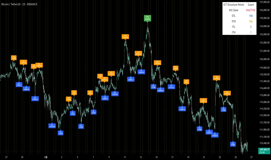
Recommendation Indicatorالوصف بالعربية
استراتيجية تداول مبنية على ٦ مؤشرات تأكيدية لرصد حركة السوق واتجاهه.
تعتمد على عدّ الشموع الصاعدة والهابطة المتتالية كعامل أساسي، وتدمج معها مؤشرات إضافية للتأكيد.
عند توافق المؤشرات معًا، يتم توليد إشارة شراء (BUY) أو بيع (SELL) واضحة على الرسم البياني.
هذا يعزز دقة الإشارات ويقلل من التذبذبات أو الإشارات الكاذبة، مما يجعلها مناسبة للمتداولين الباحثين عن قوة الاتجاه وتأكيده قبل الدخول في الصفقة.
🔎 ملاحظات الاستخدام
الاستراتيجية تحتوي على ٦ أدوات تأكيد مجتمعة لضمان إشارات أدق.
يُفضل استخدامها مع اختبار رجعي (Backtesting) قبل التداول الفعلي.
يمكن تعديل إعدادات المؤشرات لتناسب السوق أو الإطار الزمني المستخدم.
لا تعتبر توصية مالية مباشرة، وإنما أداة تعليمية وتجريبية.
---
📌 Description in English
A trading strategy built on 6 confirmation indicators to track market movements and trends.
It uses consecutive up and down bars as the core logic, combined with additional indicators for confirmation.
When all confirmations align, the strategy generates clear BUY or SELL signals on the chart.
This approach improves signal accuracy, reduces noise, and helps traders confirm market direction before entering a trade.
🔎 Usage Notes
The strategy incorporates 6 confirmation tools working together for higher accuracy.
Backtesting is recommended before applying it to live trading.
Indicator parameters can be adjusted to fit different markets and timeframes.
This is not financial advice, but an educational and experimental tool.
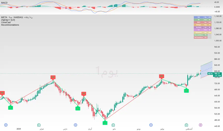

Ray Dalio's All Weather Strategy - Portfolio CalculatorTHE ALL WEATHER STRATEGY INDICATOR: A GUIDE TO RAY DALIO'S LEGENDARY PORTFOLIO APPROACH
Introduction: The Genesis of Financial Resilience
In the sprawling corridors of Bridgewater Associates, the world's largest hedge fund managing over 150 billion dollars in assets, Ray Dalio conceived what would become one of the most influential investment strategies of the modern era. The All Weather Strategy, born from decades of market observation and rigorous backtesting, represents a paradigm shift from traditional portfolio construction methods that have dominated Wall Street since Harry Markowitz's seminal work on Modern Portfolio Theory in 1952.
Unlike conventional approaches that chase returns through market timing or stock picking, the All Weather Strategy embraces a fundamental truth that has humbled countless investors throughout history: nobody can consistently predict the future direction of markets. Instead of fighting this uncertainty, Dalio's approach harnesses it, creating a portfolio designed to perform reasonably well across all economic environments, hence the evocative name "All Weather."
The strategy emerged from Bridgewater's extensive research into economic cycles and asset class behavior, culminating in what Dalio describes as "the Holy Grail of investing" in his bestselling book "Principles" (Dalio, 2017). This Holy Grail isn't about achieving spectacular returns, but rather about achieving consistent, risk-adjusted returns that compound steadily over time, much like the tortoise defeating the hare in Aesop's timeless fable.
HISTORICAL DEVELOPMENT AND EVOLUTION
The All Weather Strategy's origins trace back to the tumultuous economic periods of the 1970s and 1980s, when traditional portfolio construction methods proved inadequate for navigating simultaneous inflation and recession. Raymond Thomas Dalio, born in 1949 in Queens, New York, founded Bridgewater Associates from his Manhattan apartment in 1975, initially focusing on currency and fixed-income consulting for corporate clients.
Dalio's early experiences during the 1970s stagflation period profoundly shaped his investment philosophy. Unlike many of his contemporaries who viewed inflation and deflation as opposing forces, Dalio recognized that both conditions could coexist with either economic growth or contraction, creating four distinct economic environments rather than the traditional two-factor models that dominated academic finance.
The conceptual breakthrough came in the late 1980s when Dalio began systematically analyzing asset class performance across different economic regimes. Working with a small team of researchers, Bridgewater developed sophisticated models that decomposed economic conditions into growth and inflation components, then mapped historical asset class returns against these regimes. This research revealed that traditional portfolio construction, heavily weighted toward stocks and bonds, left investors vulnerable to specific economic scenarios.
The formal All Weather Strategy emerged in 1996 when Bridgewater was approached by a wealthy family seeking a portfolio that could protect their wealth across various economic conditions without requiring active management or market timing. Unlike Bridgewater's flagship Pure Alpha fund, which relied on active trading and leverage, the All Weather approach needed to be completely passive and unleveraged while still providing adequate diversification.
Dalio and his team spent months developing and testing various allocation schemes, ultimately settling on the 30/40/15/7.5/7.5 framework that balances risk contributions rather than dollar amounts. This approach was revolutionary because it focused on risk budgeting—ensuring that no single asset class dominated the portfolio's risk profile—rather than the traditional approach of equal dollar allocations or market-cap weighting.
The strategy's first institutional implementation began in 1996 with a family office client, followed by gradual expansion to other wealthy families and eventually institutional investors. By 2005, Bridgewater was managing over $15 billion in All Weather assets, making it one of the largest systematic strategy implementations in institutional investing.
The 2008 financial crisis provided the ultimate test of the All Weather methodology. While the S&P 500 declined by 37% and many hedge funds suffered double-digit losses, the All Weather strategy generated positive returns, validating Dalio's risk-balancing approach. This performance during extreme market stress attracted significant institutional attention, leading to rapid asset growth in subsequent years.
The strategy's theoretical foundations evolved throughout the 2000s as Bridgewater's research team, led by co-chief investment officers Greg Jensen and Bob Prince, refined the economic framework and incorporated insights from behavioral economics and complexity theory. Their research, published in numerous institutional white papers, demonstrated that traditional portfolio optimization methods consistently underperformed simpler risk-balanced approaches across various time periods and market conditions.
Academic validation came through partnerships with leading business schools and collaboration with prominent economists. The strategy's risk parity principles influenced an entire generation of institutional investors, leading to the creation of numerous risk parity funds managing hundreds of billions in aggregate assets.
In recent years, the democratization of sophisticated financial tools has made All Weather-style investing accessible to individual investors through ETFs and systematic platforms. The availability of high-quality, low-cost ETFs covering each required asset class has eliminated many of the barriers that previously limited sophisticated portfolio construction to institutional investors.
The development of advanced portfolio management software and platforms like TradingView has further democratized access to institutional-quality analytics and implementation tools. The All Weather Strategy Indicator represents the culmination of this trend, providing individual investors with capabilities that previously required teams of portfolio managers and risk analysts.
Understanding the Four Economic Seasons
The All Weather Strategy's theoretical foundation rests on Dalio's observation that all economic environments can be characterized by two primary variables: economic growth and inflation. These variables create four distinct "economic seasons," each favoring different asset classes. Rising growth benefits stocks and commodities, while falling growth favors bonds. Rising inflation helps commodities and inflation-protected securities, while falling inflation benefits nominal bonds and stocks.
This framework, detailed extensively in Bridgewater's research papers from the 1990s, suggests that by holding assets that perform well in each economic season, an investor can create a portfolio that remains resilient regardless of which season unfolds. The elegance lies not in predicting which season will occur, but in being prepared for all of them simultaneously.
Academic research supports this multi-environment approach. Ang and Bekaert (2002) demonstrated that regime changes in economic conditions significantly impact asset returns, while Fama and French (2004) showed that different asset classes exhibit varying sensitivities to economic factors. The All Weather Strategy essentially operationalizes these academic insights into a practical investment framework.
The Original All Weather Allocation: Simplicity Masquerading as Sophistication
The core All Weather portfolio, as implemented by Bridgewater for institutional clients and later adapted for retail investors, maintains a deceptively simple static allocation: 30% stocks, 40% long-term bonds, 15% intermediate-term bonds, 7.5% commodities, and 7.5% Treasury Inflation-Protected Securities (TIPS). This allocation may appear arbitrary to the uninitiated, but each percentage reflects careful consideration of historical volatilities, correlations, and economic sensitivities.
The 30% stock allocation provides growth exposure while limiting the portfolio's overall volatility. Stocks historically deliver superior long-term returns but with significant volatility, as evidenced by the Standard & Poor's 500 Index's average annual return of approximately 10% since 1926, accompanied by standard deviation exceeding 15% (Ibbotson Associates, 2023). By limiting stock exposure to 30%, the portfolio captures much of the equity risk premium while avoiding excessive volatility.
The combined 55% allocation to bonds (40% long-term plus 15% intermediate-term) serves as the portfolio's stabilizing force. Long-term bonds provide substantial interest rate sensitivity, performing well during economic slowdowns when central banks reduce rates. Intermediate-term bonds offer a balance between interest rate sensitivity and reduced duration risk. This bond-heavy allocation reflects Dalio's insight that bonds typically exhibit lower volatility than stocks while providing essential diversification benefits.
The 7.5% commodities allocation addresses inflation protection, as commodity prices typically rise during inflationary periods. Historical analysis by Bodie and Rosansky (1980) demonstrated that commodities provide meaningful diversification benefits and inflation hedging capabilities, though with considerable volatility. The relatively small allocation reflects commodities' high volatility and mixed long-term returns.
Finally, the 7.5% TIPS allocation provides explicit inflation protection through government-backed securities whose principal and interest payments adjust with inflation. Introduced by the U.S. Treasury in 1997, TIPS have proven effective inflation hedges, though they underperform nominal bonds during deflationary periods (Campbell & Viceira, 2001).
Historical Performance: The Evidence Speaks
Analyzing the All Weather Strategy's historical performance reveals both its strengths and limitations. Using monthly return data from 1970 to 2023, spanning over five decades of varying economic conditions, the strategy has delivered compelling risk-adjusted returns while experiencing lower volatility than traditional stock-heavy portfolios.
During this period, the All Weather allocation generated an average annual return of approximately 8.2%, compared to 10.5% for the S&P 500 Index. However, the strategy's annual volatility measured just 9.1%, substantially lower than the S&P 500's 15.8% volatility. This translated to a Sharpe ratio of 0.67 for the All Weather Strategy versus 0.54 for the S&P 500, indicating superior risk-adjusted performance.
More impressively, the strategy's maximum drawdown over this period was 12.3%, occurring during the 2008 financial crisis, compared to the S&P 500's maximum drawdown of 50.9% during the same period. This drawdown mitigation proves crucial for long-term wealth building, as Stein and DeMuth (2003) demonstrated that avoiding large losses significantly impacts compound returns over time.
The strategy performed particularly well during periods of economic stress. During the 1970s stagflation, when stocks and bonds both struggled, the All Weather portfolio's commodity and TIPS allocations provided essential protection. Similarly, during the 2000-2002 dot-com crash and the 2008 financial crisis, the portfolio's bond-heavy allocation cushioned losses while maintaining positive returns in several years when stocks declined significantly.
However, the strategy underperformed during sustained bull markets, particularly the 1990s technology boom and the 2010s post-financial crisis recovery. This underperformance reflects the strategy's conservative nature and diversified approach, which sacrifices potential upside for downside protection. As Dalio frequently emphasizes, the All Weather Strategy prioritizes "not losing money" over "making a lot of money."
Implementing the All Weather Strategy: A Practical Guide
The All Weather Strategy Indicator transforms Dalio's institutional-grade approach into an accessible tool for individual investors. The indicator provides real-time portfolio tracking, rebalancing signals, and performance analytics, eliminating much of the complexity traditionally associated with implementing sophisticated allocation strategies.
To begin implementation, investors must first determine their investable capital. As detailed analysis reveals, the All Weather Strategy requires meaningful capital to implement effectively due to transaction costs, minimum investment requirements, and the need for precise allocations across five different asset classes.
For portfolios below $50,000, the strategy becomes challenging to implement efficiently. Transaction costs consume a disproportionate share of returns, while the inability to purchase fractional shares creates allocation drift. Consider an investor with $25,000 attempting to allocate 7.5% to commodities through the iPath Bloomberg Commodity Index ETF (DJP), currently trading around $25 per share. This allocation targets $1,875, enough for only 75 shares, creating immediate tracking error.
At $50,000, implementation becomes feasible but not optimal. The 30% stock allocation ($15,000) purchases approximately 37 shares of the SPDR S&P 500 ETF (SPY) at current prices around $400 per share. The 40% long-term bond allocation ($20,000) buys 200 shares of the iShares 20+ Year Treasury Bond ETF (TLT) at approximately $100 per share. While workable, these allocations leave significant cash drag and rebalancing challenges.
The optimal minimum for individual implementation appears to be $100,000. At this level, each allocation becomes substantial enough for precise implementation while keeping transaction costs below 0.4% annually. The $30,000 stock allocation, $40,000 long-term bond allocation, $15,000 intermediate-term bond allocation, $7,500 commodity allocation, and $7,500 TIPS allocation each provide sufficient size for effective management.
For investors with $250,000 or more, the strategy implementation approaches institutional quality. Allocation precision improves, transaction costs decline as a percentage of assets, and rebalancing becomes highly efficient. These larger portfolios can also consider adding complexity through international diversification or alternative implementations.
The indicator recommends quarterly rebalancing to balance transaction costs with allocation discipline. Monthly rebalancing increases costs without substantial benefits for most investors, while annual rebalancing allows excessive drift that can meaningfully impact performance. Quarterly rebalancing, typically on the first trading day of each quarter, provides an optimal balance.
Understanding the Indicator's Functionality
The All Weather Strategy Indicator operates as a comprehensive portfolio management system, providing multiple analytical layers that professional money managers typically reserve for institutional clients. This sophisticated tool transforms Ray Dalio's institutional-grade strategy into an accessible platform for individual investors, offering features that rival professional portfolio management software.
The indicator's core architecture consists of several interconnected modules that work seamlessly together to provide complete portfolio oversight. At its foundation lies a real-time portfolio simulation engine that tracks the exact value of each ETF position based on current market prices, eliminating the need for manual calculations or external spreadsheets.
DETAILED INDICATOR COMPONENTS AND FUNCTIONS
Portfolio Configuration Module
The portfolio setup begins with the Portfolio Configuration section, which establishes the fundamental parameters for strategy implementation. The Portfolio Capital input accepts values from $1,000 to $10,000,000, accommodating everyone from beginning investors to institutional clients. This input directly drives all subsequent calculations, determining exact share quantities and portfolio values throughout the implementation period.
The Portfolio Start Date function allows users to specify when they began implementing the All Weather Strategy, creating a clear demarcation point for performance tracking. This feature proves essential for investors who want to track their actual implementation against theoretical performance, providing realistic assessment of strategy effectiveness including timing differences and implementation costs.
Rebalancing Frequency settings offer two options: Monthly and Quarterly. While monthly rebalancing provides more precise allocation control, quarterly rebalancing typically proves more cost-effective for most investors due to reduced transaction costs. The indicator automatically detects the first trading day of each period, ensuring rebalancing occurs at optimal times regardless of weekends, holidays, or market closures.
The Rebalancing Threshold parameter, adjustable from 0.5% to 10%, determines when allocation drift triggers rebalancing recommendations. Conservative settings like 1-2% maintain tight allocation control but increase trading frequency, while wider thresholds like 3-5% reduce trading costs but allow greater allocation drift. This flexibility accommodates different risk tolerances and cost structures.
Visual Display System
The Show All Weather Calculator toggle controls the main dashboard visibility, allowing users to focus on chart visualization when detailed metrics aren't needed. When enabled, this comprehensive dashboard displays current portfolio value, individual ETF allocations, target versus actual weights, rebalancing status, and performance metrics in a professionally formatted table.
Economic Environment Display provides context about current market conditions based on growth and inflation indicators. While simplified compared to Bridgewater's sophisticated regime detection, this feature helps users understand which economic "season" currently prevails and which asset classes should theoretically benefit.
Rebalancing Signals illuminate when portfolio drift exceeds user-defined thresholds, highlighting specific ETFs that require adjustment. These signals use color coding to indicate urgency: green for balanced allocations, yellow for moderate drift, and red for significant deviations requiring immediate attention.
Advanced Label System
The rebalancing label system represents one of the indicator's most innovative features, providing three distinct detail levels to accommodate different user needs and experience levels. The "None" setting displays simple symbols marking portfolio start and rebalancing events without cluttering the chart with text. This minimal approach suits experienced investors who understand the implications of each symbol.
"Basic" label mode shows essential information including portfolio values at each rebalancing point, enabling quick assessment of strategy performance over time. These labels display "START $X" for portfolio initiation and "RBL $Y" for rebalancing events, providing clear performance tracking without overwhelming detail.
"Detailed" labels provide comprehensive trading instructions including exact buy and sell quantities for each ETF. These labels might display "RBL $125,000 BUY 15 SPY SELL 25 TLT BUY 8 IEF NO TRADES DJP SELL 12 SCHP" providing complete implementation guidance. This feature essentially transforms the indicator into a personal portfolio manager, eliminating guesswork about exact trades required.
Professional Color Themes
Eight professionally designed color themes adapt the indicator's appearance to different aesthetic preferences and market analysis styles. The "Gold" theme reflects traditional wealth management aesthetics, while "EdgeTools" provides modern professional appearance. "Behavioral" uses psychologically informed colors that reinforce disciplined decision-making, while "Quant" employs high-contrast combinations favored by quantitative analysts.
"Ocean," "Fire," "Matrix," and "Arctic" themes provide distinctive visual identities for traders who prefer unique chart aesthetics. Each theme automatically adjusts for dark or light mode optimization, ensuring optimal readability across different TradingView configurations.
Real-Time Portfolio Tracking
The portfolio simulation engine continuously tracks five separate ETF positions: SPY for stocks, TLT for long-term bonds, IEF for intermediate-term bonds, DJP for commodities, and SCHP for TIPS. Each position's value updates in real-time based on current market prices, providing instant feedback about portfolio performance and allocation drift.
Current share calculations determine exact holdings based on the most recent rebalancing, while target shares reflect optimal allocation based on current portfolio value. Trade calculations show precisely how many shares to buy or sell during rebalancing, eliminating manual calculations and potential errors.
Performance Analytics Suite
The indicator's performance measurement capabilities rival professional portfolio analysis software. Sharpe ratio calculations incorporate current risk-free rates obtained from Treasury yield data, providing accurate risk-adjusted performance assessment. Volatility measurements use rolling periods to capture changing market conditions while maintaining statistical significance.
Portfolio return calculations track both absolute and relative performance, comparing the All Weather implementation against individual asset classes and benchmark indices. These metrics update continuously, providing real-time assessment of strategy effectiveness and implementation quality.
Data Quality Monitoring
Sophisticated data quality checks ensure reliable indicator operation across different market conditions and potential data interruptions. The system monitors all five ETF price feeds plus economic data sources, providing quality scores that alert users to potential data issues that might affect calculations.
When data quality degrades, the indicator automatically switches to fallback values or alternative data sources, maintaining functionality during temporary market data interruptions. This robust design ensures consistent operation even during volatile market conditions when data feeds occasionally experience disruptions.
Risk Management and Behavioral Considerations
Despite its sophisticated design, the All Weather Strategy faces behavioral challenges that have derailed countless well-intentioned investment plans. The strategy's conservative nature means it will underperform growth stocks during bull markets, potentially by substantial margins. Maintaining discipline during these periods requires understanding that the strategy optimizes for risk-adjusted returns over absolute returns.
Behavioral finance research by Kahneman and Tversky (1979) demonstrates that investors feel losses approximately twice as intensely as equivalent gains. This loss aversion creates powerful psychological pressure to abandon defensive strategies during bull markets when aggressive portfolios appear more attractive. The All Weather Strategy's bond-heavy allocation will seem overly conservative when technology stocks double in value, as occurred repeatedly during the 2010s.
Conversely, the strategy's defensive characteristics provide psychological comfort during market stress. When stocks crash 30-50%, as they periodically do, the All Weather portfolio's modest losses feel manageable rather than catastrophic. This emotional stability enables investors to maintain their investment discipline when others capitulate, often at the worst possible times.
Rebalancing discipline presents another behavioral challenge. Selling winners to buy losers contradicts natural human tendencies but remains essential for the strategy's success. When stocks have outperformed bonds for several quarters, rebalancing requires selling high-performing stock positions to purchase seemingly stagnant bond positions. This action feels counterintuitive but captures the strategy's systematic approach to risk management.
Tax considerations add complexity for taxable accounts. Frequent rebalancing generates taxable events that can erode after-tax returns, particularly for high-income investors facing elevated capital gains rates. Tax-advantaged accounts like 401(k)s and IRAs provide ideal vehicles for All Weather implementation, eliminating tax friction from rebalancing activities.
Capital Requirements and Cost Analysis
Comprehensive cost analysis reveals the capital requirements for effective All Weather implementation. Annual expenses include management fees for each ETF, transaction costs from rebalancing, and bid-ask spreads from trading less liquid securities.
ETF expense ratios vary significantly across asset classes. The SPDR S&P 500 ETF charges 0.09% annually, while the iShares 20+ Year Treasury Bond ETF charges 0.20%. The iShares 7-10 Year Treasury Bond ETF charges 0.15%, the Schwab US TIPS ETF charges 0.05%, and the iPath Bloomberg Commodity Index ETF charges 0.75%. Weighted by the All Weather allocations, total expense ratios average approximately 0.19% annually.
Transaction costs depend heavily on broker selection and account size. Premium brokers like Interactive Brokers charge $1-2 per trade, resulting in $20-40 annually for quarterly rebalancing. Discount brokers may charge higher per-trade fees but offer commission-free ETF trading for selected funds. Zero-commission brokers eliminate explicit trading costs but often impose wider bid-ask spreads that function as hidden fees.
Bid-ask spreads represent the difference between buying and selling prices for each security. Highly liquid ETFs like SPY maintain spreads of 1-2 basis points, while less liquid commodity ETFs may exhibit spreads of 5-10 basis points. These costs accumulate through rebalancing activities, typically totaling 10-15 basis points annually.
For a $100,000 portfolio, total annual costs including expense ratios, transaction fees, and spreads typically range from 0.35% to 0.45%, or $350-450 annually. These costs decline as a percentage of assets as portfolio size increases, reaching approximately 0.25% for portfolios exceeding $250,000.
Comparing costs to potential benefits reveals the strategy's value proposition. Historical analysis suggests the All Weather approach reduces portfolio volatility by 35-40% compared to stock-heavy allocations while maintaining competitive returns. This volatility reduction provides substantial value during market stress, potentially preventing behavioral mistakes that destroy long-term wealth.
Alternative Implementations and Customizations
While the original All Weather allocation provides an excellent starting point, investors may consider modifications based on personal circumstances, market conditions, or geographic considerations. International diversification represents one potential enhancement, adding exposure to developed and emerging market bonds and equities.
Geographic customization becomes important for non-US investors. European investors might replace US Treasury bonds with German Bunds or broader European government bond indices. Currency hedging decisions add complexity but may reduce volatility for investors whose spending occurs in non-dollar currencies.
Tax-location strategies optimize after-tax returns by placing tax-inefficient assets in tax-advantaged accounts while holding tax-efficient assets in taxable accounts. TIPS and commodity ETFs generate ordinary income taxed at higher rates, making them candidates for retirement account placement. Stock ETFs generate qualified dividends and long-term capital gains taxed at lower rates, making them suitable for taxable accounts.
Some investors prefer implementing the bond allocation through individual Treasury securities rather than ETFs, eliminating management fees while gaining precise maturity control. Treasury auctions provide access to new securities without bid-ask spreads, though this approach requires more sophisticated portfolio management.
Factor-based implementations replace broad market ETFs with factor-tilted alternatives. Value-tilted stock ETFs, quality-focused bond ETFs, or momentum-based commodity indices may enhance returns while maintaining the All Weather framework's diversification benefits. However, these modifications introduce additional complexity and potential tracking error.
Conclusion: Embracing the Long Game
The All Weather Strategy represents more than an investment approach; it embodies a philosophy of financial resilience that prioritizes sustainable wealth building over speculative gains. In an investment landscape increasingly dominated by algorithmic trading, meme stocks, and cryptocurrency volatility, Dalio's methodical approach offers a refreshing alternative grounded in economic theory and historical evidence.
The strategy's greatest strength lies not in its potential for extraordinary returns, but in its capacity to deliver reasonable returns across diverse economic environments while protecting capital during market stress. This characteristic becomes increasingly valuable as investors approach or enter retirement, when portfolio preservation assumes greater importance than aggressive growth.
Implementation requires discipline, adequate capital, and realistic expectations. The strategy will underperform growth-oriented approaches during bull markets while providing superior downside protection during bear markets. Investors must embrace this trade-off consciously, understanding that the strategy optimizes for long-term wealth building rather than short-term performance.
The All Weather Strategy Indicator democratizes access to institutional-quality portfolio management, providing individual investors with tools previously available only to wealthy families and institutions. By automating allocation tracking, rebalancing signals, and performance analysis, the indicator removes much of the complexity that has historically limited sophisticated strategy implementation.
For investors seeking a systematic, evidence-based approach to long-term wealth building, the All Weather Strategy provides a compelling framework. Its emphasis on diversification, risk management, and behavioral discipline aligns with the fundamental principles that have created lasting wealth throughout financial history. While the strategy may not generate headlines or inspire cocktail party conversations, it offers something more valuable: a reliable path toward financial security across all economic seasons.
As Dalio himself notes, "The biggest mistake investors make is to believe that what happened in the recent past is likely to persist, and they design their portfolios accordingly." The All Weather Strategy's enduring appeal lies in its rejection of this recency bias, instead embracing the uncertainty of markets while positioning for success regardless of which economic season unfolds.
STEP-BY-STEP INDICATOR SETUP GUIDE
Setting up the All Weather Strategy Indicator requires careful attention to each configuration parameter to ensure optimal implementation. This comprehensive setup guide walks through every setting and explains its impact on strategy performance.
Initial Setup Process
Begin by adding the indicator to your TradingView chart. Search for "Ray Dalio's All Weather Strategy" in the indicator library and apply it to any chart. The indicator operates independently of the underlying chart symbol, drawing data directly from the five required ETFs regardless of which security appears on the chart.
Portfolio Configuration Settings
Start with the Portfolio Capital input, which drives all subsequent calculations. Enter your exact investable capital, ranging from $1,000 to $10,000,000. This input determines share quantities, trade recommendations, and performance calculations. Conservative recommendations suggest minimum capitals of $50,000 for basic implementation or $100,000 for optimal precision.
Select your Portfolio Start Date carefully, as this establishes the baseline for all performance calculations. Choose the date when you actually began implementing the All Weather Strategy, not when you first learned about it. This date should reflect when you first purchased ETFs according to the target allocation, creating realistic performance tracking.
Choose your Rebalancing Frequency based on your cost structure and precision preferences. Monthly rebalancing provides tighter allocation control but increases transaction costs. Quarterly rebalancing offers the optimal balance for most investors between allocation precision and cost control. The indicator automatically detects appropriate trading days regardless of your selection.
Set the Rebalancing Threshold based on your tolerance for allocation drift and transaction costs. Conservative investors preferring tight control should use 1-2% thresholds, while cost-conscious investors may prefer 3-5% thresholds. Lower thresholds maintain more precise allocations but trigger more frequent trading.
Display Configuration Options
Enable Show All Weather Calculator to display the comprehensive dashboard containing portfolio values, allocations, and performance metrics. This dashboard provides essential information for portfolio management and should remain enabled for most users.
Show Economic Environment displays current economic regime classification based on growth and inflation indicators. While simplified compared to Bridgewater's sophisticated models, this feature provides useful context for understanding current market conditions.
Show Rebalancing Signals highlights when portfolio allocations drift beyond your threshold settings. These signals use color coding to indicate urgency levels, helping prioritize rebalancing activities.
Advanced Label Customization
Configure Show Rebalancing Labels based on your need for chart annotations. These labels mark important portfolio events and can provide valuable historical context, though they may clutter charts during extended time periods.
Select appropriate Label Detail Levels based on your experience and information needs. "None" provides minimal symbols suitable for experienced users. "Basic" shows portfolio values at key events. "Detailed" provides complete trading instructions including exact share quantities for each ETF.
Appearance Customization
Choose Color Themes based on your aesthetic preferences and trading style. "Gold" reflects traditional wealth management appearance, while "EdgeTools" provides modern professional styling. "Behavioral" uses psychologically informed colors that reinforce disciplined decision-making.
Enable Dark Mode Optimization if using TradingView's dark theme for optimal readability and contrast. This setting automatically adjusts all colors and transparency levels for the selected theme.
Set Main Line Width based on your chart resolution and visual preferences. Higher width values provide clearer allocation lines but may overwhelm smaller charts. Most users prefer width settings of 2-3 for optimal visibility.
Troubleshooting Common Setup Issues
If the indicator displays "Data not available" messages, verify that all five ETFs (SPY, TLT, IEF, DJP, SCHP) have valid price data on your selected timeframe. The indicator requires daily data availability for all components.
When rebalancing signals seem inconsistent, check your threshold settings and ensure sufficient time has passed since the last rebalancing event. The indicator only triggers signals on designated rebalancing days (first trading day of each period) when drift exceeds threshold levels.
If labels appear at unexpected chart locations, verify that your chart displays percentage values rather than price values. The indicator forces percentage formatting and 0-40% scaling for optimal allocation visualization.
COMPREHENSIVE BIBLIOGRAPHY AND FURTHER READING
PRIMARY SOURCES AND RAY DALIO WORKS
Dalio, R. (2017). Principles: Life and work. New York: Simon & Schuster.
Dalio, R. (2018). A template for understanding big debt crises. Bridgewater Associates.
Dalio, R. (2021). Principles for dealing with the changing world order: Why nations succeed and fail. New York: Simon & Schuster.
BRIDGEWATER ASSOCIATES RESEARCH PAPERS
Jensen, G., Kertesz, A. & Prince, B. (2010). All Weather strategy: Bridgewater's approach to portfolio construction. Bridgewater Associates Research.
Prince, B. (2011). An in-depth look at the investment logic behind the All Weather strategy. Bridgewater Associates Daily Observations.
Bridgewater Associates. (2015). Risk parity in the context of larger portfolio construction. Institutional Research.
ACADEMIC RESEARCH ON RISK PARITY AND PORTFOLIO CONSTRUCTION
Ang, A. & Bekaert, G. (2002). International asset allocation with regime shifts. The Review of Financial Studies, 15(4), 1137-1187.
Bodie, Z. & Rosansky, V. I. (1980). Risk and return in commodity futures. Financial Analysts Journal, 36(3), 27-39.
Campbell, J. Y. & Viceira, L. M. (2001). Who should buy long-term bonds? American Economic Review, 91(1), 99-127.
Clarke, R., De Silva, H. & Thorley, S. (2013). Risk parity, maximum diversification, and minimum variance: An analytic perspective. Journal of Portfolio Management, 39(3), 39-53.
Fama, E. F. & French, K. R. (2004). The capital asset pricing model: Theory and evidence. Journal of Economic Perspectives, 18(3), 25-46.
BEHAVIORAL FINANCE AND IMPLEMENTATION CHALLENGES
Kahneman, D. & Tversky, A. (1979). Prospect theory: An analysis of decision under risk. Econometrica, 47(2), 263-292.
Thaler, R. H. & Sunstein, C. R. (2008). Nudge: Improving decisions about health, wealth, and happiness. New Haven: Yale University Press.
Montier, J. (2007). Behavioural investing: A practitioner's guide to applying behavioural finance. Chichester: John Wiley & Sons.
MODERN PORTFOLIO THEORY AND QUANTITATIVE METHODS
Markowitz, H. (1952). Portfolio selection. The Journal of Finance, 7(1), 77-91.
Sharpe, W. F. (1964). Capital asset prices: A theory of market equilibrium under conditions of risk. The Journal of Finance, 19(3), 425-442.
Black, F. & Litterman, R. (1992). Global portfolio optimization. Financial Analysts Journal, 48(5), 28-43.
PRACTICAL IMPLEMENTATION AND ETF ANALYSIS
Gastineau, G. L. (2010). The exchange-traded funds manual. 2nd ed. Hoboken: John Wiley & Sons.
Poterba, J. M. & Shoven, J. B. (2002). Exchange-traded funds: A new investment option for taxable investors. American Economic Review, 92(2), 422-427.
Israelsen, C. L. (2005). A refinement to the Sharpe ratio and information ratio. Journal of Asset Management, 5(6), 423-427.
ECONOMIC CYCLE ANALYSIS AND ASSET CLASS RESEARCH
Ilmanen, A. (2011). Expected returns: An investor's guide to harvesting market rewards. Chichester: John Wiley & Sons.
Swensen, D. F. (2009). Pioneering portfolio management: An unconventional approach to institutional investment. Rev. ed. New York: Free Press.
Siegel, J. J. (2014). Stocks for the long run: The definitive guide to financial market returns & long-term investment strategies. 5th ed. New York: McGraw-Hill Education.
RISK MANAGEMENT AND ALTERNATIVE STRATEGIES
Taleb, N. N. (2007). The black swan: The impact of the highly improbable. New York: Random House.
Lowenstein, R. (2000). When genius failed: The rise and fall of Long-Term Capital Management. New York: Random House.
Stein, D. M. & DeMuth, P. (2003). Systematic withdrawal from retirement portfolios: The impact of asset allocation decisions on portfolio longevity. AAII Journal, 25(7), 8-12.
CONTEMPORARY DEVELOPMENTS AND FUTURE DIRECTIONS
Asness, C. S., Frazzini, A. & Pedersen, L. H. (2012). Leverage aversion and risk parity. Financial Analysts Journal, 68(1), 47-59.
Roncalli, T. (2013). Introduction to risk parity and budgeting. Boca Raton: CRC Press.
Ibbotson Associates. (2023). Stocks, bonds, bills, and inflation 2023 yearbook. Chicago: Morningstar.
PERIODICALS AND ONGOING RESEARCH
Journal of Portfolio Management - Quarterly publication featuring cutting-edge research on portfolio construction and risk management
Financial Analysts Journal - Bi-monthly publication of the CFA Institute with practical investment research
Bridgewater Associates Daily Observations - Regular market commentary and research from the creators of the All Weather Strategy
RECOMMENDED READING SEQUENCE
For investors new to the All Weather Strategy, begin with Dalio's "Principles" for philosophical foundation, then proceed to the Bridgewater research papers for technical details. Supplement with Markowitz's original portfolio theory work and behavioral finance literature from Kahneman and Tversky.
Intermediate students should focus on academic papers by Ang & Bekaert on regime shifts, Clarke et al. on risk parity methods, and Ilmanen's comprehensive analysis of expected returns across asset classes.
Advanced practitioners will benefit from Roncalli's technical treatment of risk parity mathematics, Asness et al.'s academic critique of leverage aversion, and ongoing research in the Journal of Portfolio Management.
