Yield Curve Phase Signal - Macro OpticsThe Yield Curve Phase Signal identifies where we are in the 10s–2s curve by detecting pivots and classifying each span as Bull Steepening, Bear Steepening, Bear Flattening, or Bull Flattening with clear background shading and date labels.
A live table tracks 10-year and 2-year yield performance across current, previous, 1-week, 1-month, and 3-month windows, plus the curve delta, so you can see phase shifts in real time.
Use the chart, table, and the Yield Curve Phase Signal PDF presentation slides together to spot regime transitions that tend to precede rotations across equities, rates, and risk assets.
To get your copy of the pdf slides that go with this indicator, go to macro-optics.com
Forecasting

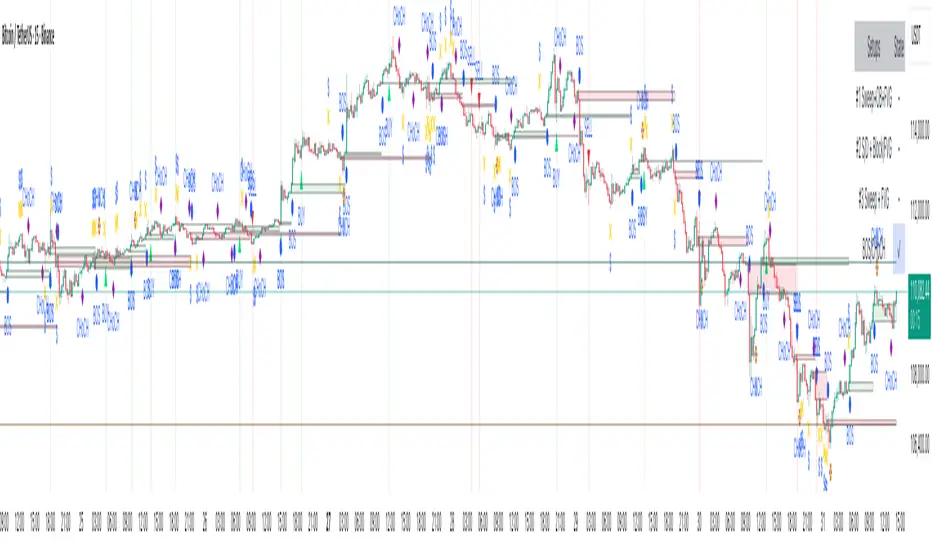
Smart Risk - Three Institutional Models📘 Smart Risk – Three Institutional Entry Models
A precision-engineered institutional framework that blends liquidity, structure, and multi-time-frame confirmation.
🧠 Concept Overview
The Smart Risk indicator models how institutional traders and algorithms engineer entries around liquidity, imbalance, and structural shifts .
It unifies t hree distinct institutional entry models —each built around core Smart Money Concepts (SMC)—and enhances them with a Multi-Time-Frame Confluence (MTF) engine for directional alignment.
This tool doesn’t simply merge indicators.
It connects l iquidity sweeps, order-block reactions, breaker validation, and fair-value-gap mitigation into one cohesive trading logic—filtering every setup through trend, structure, and volume confirmation.
⚙️ How It Works
Setup #1 – Liquidity Sweep + Order Block Revisit + FVG Mitigation
Identifies engineered stop-hunts where price sweeps external liquidity and returns to a prior Order Block or Fair Value Gap (FVG).
Signals reversal-style entries with high probability of mean-reversion or mitigation.
Setup #2 – Supply/Demand + Mitigation / Breaker / FVG Continuation
Captures continuation trades inside trending structure.
When trend bias (via moving-average context) aligns with breaker or mitigation blocks, signals confirm institutional continuation sequences.
Setup #3 – Sweep + Classic FVG Reaction
Tracks clean displacement gaps following a liquidity sweep—ideal for scalpers and intraday reversals where imbalances act as magnets for price.
Each setup can be independently enabled or disabled from the panel.
A built-in signal-cooldown prevents repetitive triggers on the same leg.
🕒 Multi-Time-Frame Confluence
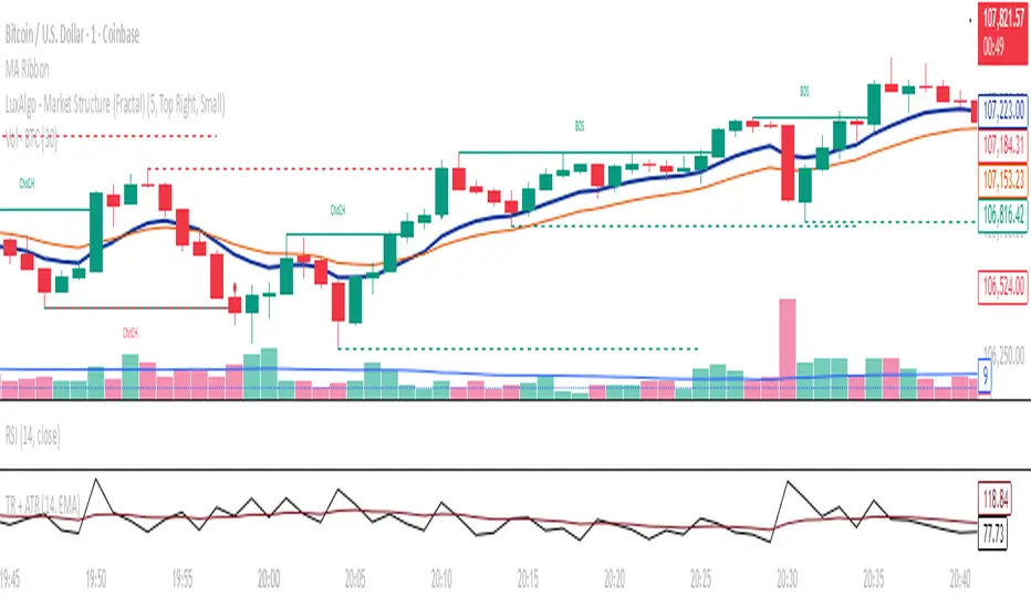
The new MTF module aligns lower-time-frame precision entries with higher-time-frame market structure.
When enabled, each setup only validates if the HTF trend confirms the same directional bias as the LTF pattern—e.g. a 5-minute bullish FVG signal requires a bullish 1-hour structure.
This ensures institutional logic respects global liquidity flow and avoids counter-trend traps.
MTF Controls:
• ✅ Enable MTF Confluence toggle
• ⏱️ Lower Time-Frame (LTF) selector (default 5 min)
• ⏱️ Higher Time-Frame (HTF) selector (default 1 hour)
• 🔄 Automatic SMA-based HTF trend detection
🎨 Visualization & Dashboard
• Order Block / Supply–Demand Zones — highlight institutional footprints
• Fair Value Gaps (FVGs) — reveal displacement inefficiencies
• Liquidity Sweeps (X / $) — mark engineered stops
• BOS & CHoCH — confirm structure continuation or reversal
• Compact Dashboard — live “Armed” state for each setup and MTF bias
Color-coded background cues emphasize active trade phases without clutter.
🧩 Core Algorithm Highlights
• Dynamic swing and pivot structure detection
• Breaker / Mitigation / Volume confirmation filters
• Fair-Value-Gap logic with directional alignment
• Cooldown control for signal throttling
• Multi-Time-Frame bias filter for contextual precision
⸻
📈 How to Use
1. Apply indicator to any asset or timeframe.
2. Select which institutional setups you want active.
3. Optionally enable MTF Confluence (5 min → 1 hr recommended).
4. Wait for BOS/CHoCH confirmation + zone alignment before entry.
5. Use OB and FVG zones for entry/exit planning with risk management.
⸻
💡 Originality Statement
This script introduces a multi-layered institutional logic engine that merges liquidity, mitigation, and imbalance behavior into a unified framework—augmented with time-frame synchronization and signal-cooldown management.
All logic, calculations, and visualization structure were built from scratch for this model.
It is not a mash-up of existing public indicators and offers measurable analytical value through MTF-aware trade validation.
⸻
⚠️ Disclaimer
This tool is intended for educational and analytical purposes only.
It does not provide financial advice or guaranteed trading outcomes.
Always back-test, validate setups, and apply proper risk management.
Volatility Cones **Volatility Cones - Interactive**
This indicator visualizes volatility cones based on historical or manual volatility and projects them up to 252 trading days into the future.
**Features:**
- Automatic start at the first trading day of the year (customizable)
- Volatility calculation from historical data or manual input
- Display of ±1σ, ±2σ, and ±3σ bands
- Projection of expected price movements based on volatility
**Use Case:**
Ideal for options traders and risk management to assess expected price movements over different time horizons.

EMA 20/50/100/200 Multi-Layer Trend Panel 📘 EMA 20/50/100/200 Multi-Layer Trend Panel
A clean and advanced trend structure analyzer designed to help traders monitor short-, medium-, and long-term market momentum simultaneously.
This indicator combines four key EMAs — 20, 50, 100, and 200 — with visual clouds, dynamic color coding, crossover labels, and a powerful real-time summary panel.
🔍 How It Works
Each EMA line changes color depending on its slope direction
→ Green tone = uptrend, Red tone = downtrend.
Detects and labels important crossovers automatically:
20/50 GC → Short-term bullish shift (Golden Cross).
50/200 GC → Long-term strong bullish breakout.
DC labels indicate Death Cross or bearish reversals.
Cloud zones between EMAs visualize the interaction between short- and long-term trends.
A compact top-right panel displays each EMA’s current value, slope direction, and overall trend alignment status (BULL / BEAR / MIXED).
⚙️ Advantages
✅ Tracks trend structure on multiple layers (short → medium → long).
✅ Highlights momentum shifts using dynamic EMA slope coloring.
✅ Provides early visual warnings of trend reversals (GC/DC).
✅ Clean, minimal panel offers an instant multi-EMA overview.
✅ Compatible with multi-timeframe (MTF) analysis — view higher-TF EMAs within lower charts.
✅ Optional bar and background coloring makes trend zones easy to interpret.
💡 Pro Tips
On higher timeframes (1D / 4H), the 50/200 cross defines the macro market direction.
On lower timeframes (5m – 15m), the 20/50 cross helps refine entry timing.
When the panel shows
→ Aligned BULL (20>50>100>200) → Strong trending condition.
→ Mixed → Ranging or transition phase.
Combine with volume or RSI for confluence in entry/exit decisions.
🧭 Purpose
This indicator aims to simplify complex market structure into an elegant, color-coded system — allowing traders to stay aligned with the dominant trend while spotting early reversals across multiple time horizons.
🧩 Ideal For
Swing & position traders confirming long-term bias.
Intraday traders aligning entries with higher-TF EMAs.
Strategy developers seeking multi-EMA trend filters.
Anyone who wants a clean, informative, and unobtrusive visual trend dashboard.
⚠️ Notes
The script supports optional MTF (multi-timeframe) mode — use carefully, as MTF data may repaint during incomplete bars.
No trading system is perfect; always combine with your personal strategy and proper risk management.

8x Heikin Ashi Streak (1m) by Bitcoin Benito🧭 Indicator Description: “8x Heikin Ashi Streak (1m) by Bitcoin Benito”
**Purpose:**
The *8x Heikin Ashi Streak* indicator helps traders quickly identify strong short-term momentum on the **1-minute timeframe**. It automatically tracks Heikin Ashi candles and alerts you whenever **8 consecutive bullish or bearish candles** appear — a visual cue that a strong intraday trend or exhaustion point might be forming.
---
🔍 **How It Works**
* The indicator continuously counts Heikin Ashi candles in real-time.
* When it detects **8 bullish (green)** or **8 bearish (red)** candles in a row:
* A green ▲ marker appears **below** the 8th candle for bullish streaks.
* A red ▼ marker appears **above** the 8th candle for bearish streaks.
* You can set alerts to automatically notify you when these streaks occur.
This makes it ideal for **momentum traders**, **scalpers**, and **trend-reversal spotters** who want to:
* Catch strong intraday moves early.
* Identify potential overextension zones before pullbacks.
* Automate alert signals for short-term trading setups.
IMPORTANT: Only trade when most of the 8 candles are below/above the EMA 8 Line respectively. Add an EMA 8 indicator to see if this is the case
---
⚙️ **How to Use**
1. **Apply to a 1-minute chart** (this script is optimized for 1m timeframes).
2. When the indicator plots a green or red triangle:
* **Green triangle (8 bullish candles):** Trend momentum is strong upward.
* **Red triangle (8 bearish candles):** Downward momentum is dominant.
3. Optionally, combine with volume or EMA filters to confirm breakouts or exhaustion.
---
🔔 **Setting Up Alerts**
* Click the **Alert (🔔)** icon on TradingView.
* Under *Condition*, select:
* “8x Heikin Ashi Streak (1m)” → “8 Bullish Heikin Ashi (1m)”
* OR “8x Heikin Ashi Streak (1m)” → “8 Bearish Heikin Ashi (1m)”
* Choose **Once per bar close** to trigger the alert when the 8th candle completes.
* Add your custom message, e.g.
> “🚀 8 bullish Heikin Ashi candles in a row on 1-minute chart!”
> “🔻 8 bearish Heikin Ashi candles in a row on 1-minute chart!”
---
📊 **Best Practices**
* Works best on **liquid assets** (major forex pairs, indices, BTC/USD, etc.).
* Pair with **RSI**, **EMA**, or **Volume** indicators for stronger confirmation.
* Not a standalone buy/sell signal — treat it as a **momentum or exhaustion alert**.
* Can be adapted to other timeframes by changing chart resolution.
---
⚠️ **Disclaimer**
This indicator is for **educational and analytical purposes only**.
Trading carries risk — always test on demo accounts and use proper risk management.
No indicator guarantees profit; this is a tool for insight and timing, not financial advice.

True Range(TR) & ATR Combined – Volatility Strength IndicatorThis indicator combines True Range (TR) and Average True Range (ATR) into a single panel for a clearer understanding of price volatility.
True Range (TR) measures the absolute price movement between highs, lows, and previous closes — showing raw, unsmoothed volatility.
Average True Range (ATR) is a moving average of the True Range, providing a smoother, more stable volatility signal.
📊 Usage Tips:
High TR/ATR values indicate strong price movement or volatility expansion.
Low values suggest compression or a potential volatility breakout zone.
Can be used for stop-loss placement, volatility filters, or trend strength confirmation.
⚙️ Features:
Multiple smoothing methods: RMA, SMA, EMA, WMA.
Adjustable ATR length.
Separate colored plots for TR (yellow) and ATR (red).
Works across all timeframes and instruments.
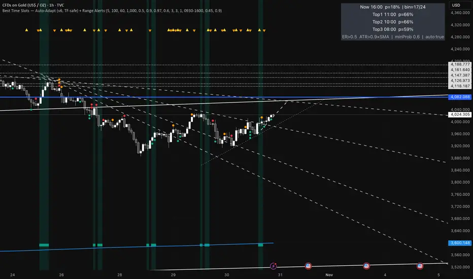
Best Time Slots — Auto-Adapt (v6, TF-safe) + Range AlertsTime & binning
Auto-adapt to timeframe
Makes all time windows scale to your chart’s bar size (so it “just works” on 1m, 15m, 4H, Daily).
• On = recommended. • Off = fixed default lengths.
Minimum Bin (minutes)
The size of each daily time slot we track (e.g., 5-min bins). The script uses the larger of this and your bar size.
• Higher = fewer, broader slots; smoother stats. • Lower = more, narrower slots; needs more history.
• Try: 5–15 on intraday, 60–240 on higher TFs.
Lookback windows (used when Auto-adapt = ON)
Target ER Window (minutes)
How far back we look to judge Efficiency Ratio (how “straight” the move was).
• Higher = stricter/smoother; fewer bars qualify as “movement”. • Lower = more sensitive.
• Try: 60–120 min intraday; 240–600 min for higher TFs.
Target ATR Window (minutes)
How far back we compute ATR (typical range).
• Higher = steadier ATR baseline. • Lower = reacts faster.
• Try: 30–120 min intraday; 240–600 min higher TFs.
Target Normalization Window (minutes)
How far back for the average ATR (the baseline we compare to).
• Higher = stricter “above average range” check. • Lower = easier to pass.
• Try: ~500–1500 min.
What counts as “movement”
ER Threshold (0–1)
Minimum efficiency a bar must have to count as movement.
• Higher = only very “clean, one-direction” bars count. • Lower = more bars count.
• Try: 0.55–0.65. (0.60 = balanced.)
ATR Floor vs SMA(ATR)
Requires range to be at least this many × average ATR.
• Higher (e.g., 1.2) = demand bigger-than-usual ranges. • Lower (e.g., 0.9) = allow smaller ranges.
• Try: 1.0 (above average).
How history is averaged
Recent Days Weight (per-day decay)
Gives more weight to recent days. Example: 0.97 ≈ each day old counts ~3% less.
• Higher (0.99) = slower fade (older days matter more). • Lower (0.95) = faster fade.
• Try: 0.97–0.99.
Laplace Prior Seen / Laplace Prior Hit
“Starter counts” so early stats aren’t crazy when you have little data.
• Higher priors = probabilities start closer to average; need more real data to move.
• Try: Seen=3, Hit=1 (defaults).
Min Samples (effective)
Don’t highlight a slot unless it has at least this many effective samples (after decay + priors).
• Higher = safer, but fewer highlights early.
• Try: 3–10.
When to highlight on the chart
Min Probability to Highlight
We shade/mark bars only if their slot’s historical movement probability is ≥ this.
• Higher = pickier, fewer highlights. • Lower = more highlights.
• Try: 0.45–0.60.
Show Markers on Good Bins
Draws a small square on bars that fall in a “good” slot (in addition to the soft background).
Limit to market hours (optional)
Restrict to Session + Session
Only learn/score inside this time window (e.g., “0930-1600”). Uses the chart/exchange timezone.
• Turn on if you only care about RTH.
Range (chop) alerts
Range START if ER ≤
Triggers range when efficiency drops below this level (price starts zig-zagging).
• Higher = easier to call “range”. • Lower = stricter.
Range START if ATR ≤ this × SMA(ATR)
Also triggers range when ATR shrinks below this fraction of its average (volatility contraction).
• Higher (e.g., 1.0) = stricter (must be at/under average). • Lower (e.g., 0.9) = easier to call range.
Alerts on bar close
If ON, alerts fire once per bar close (cleaner). If OFF, they can trigger intrabar (faster, noisier).
Quick “what happens if I change X?”
Want more highlighted times? ↓ Min Probability, ↓ ER Threshold, or ↓ ATR Floor (e.g., 0.9).
Want stricter highlights? ↑ Min Probability, ↑ ER Threshold, or ↑ ATR Floor (e.g., 1.2).
Want recent days to matter more? ↑ Recent Days Weight toward 0.99.
On 4H/Daily, widen Minimum Bin (e.g., 60–240) and maybe lower Min Probability a bit.
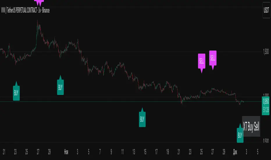
XT Buy Sell v1.0 Lite: Non-Repainting Signal Indicator🚀 XT Buy Sell v1.0 Lite: Non-Repainting Signal Indicator
The XT Buy Sell v1.0 Lite indicator is a streamlined version of our flagship tool, designed for traders who need a reliable, ready-to-use source of signals for market entry and exit.
✨ Key Advantages
Non-Repainting Signals: BUY/SELL signals remain permanently on the chart, providing reliability and easy verification on historical data.
High Accuracy: Developed as one of the most accurate tools for identifying entry points.
Ready "Out of the Box": The indicator comes with optimal default settings. All additional and advanced settings are available in the PRO version.
Versatility: Suitable for both Spot and Futures/Leveraged trading.
🔔 Convenience Features
Alerts: Set up alerts for BUY/SELL signals so you don't have to constantly monitor the chart.
Optimization: Configure alerts on the specific coins (tickers) where the indicator shows the best setups (most accurate and profitable).
🧠 Recommendations for Professional Trading (Risk Management)
To achieve maximum results and safety, follow these guidelines:
Historical Backtesting: Always verify the indicator's performance on the history of the selected trading pair before deployment.
Multi-Timeframe Analysis: Utilize the principle of "Signal on Lower TF, Confirmation on Higher TF" to increase your trading confidence.
Entry Confirmation: For maximum entry precision, it is recommended to use it in conjunction with our additional tool "X Trend Dashboard (Lite)".
Sequential Signals: The consecutive appearance of signals in the same direction (e.g., two or more consecutive BUYS) can be interpreted as a signal for re-entry/averaging down the position.
Risk Management:
Always set Stop-Losses.
Move the trade to Break-Even as soon as possible.
Carefully consider the risks and the leverage being used.
Happy trading and profits to all! 📈💰
Pullback Levels from ATH# ATH Pullback Levels
**Assess correction depth with precision – 5%, 10%, 15%, 20% below All-Time High**
---
### Overview
This indicator draws **horizontal support lines** at **5%, 10%, 15%, and 20%** below the **All-Time High (ATH)** of any asset. Perfect for **swing traders**, **long-term investors**, and **bull market participants** who want to:
- Measure **pullback depth** in real-time
- Identify **potential support zones**
- Set **alerts** when price enters key retracement levels
---
### Features
| Feature | Description |
|--------|-------------|
| **Dynamic ATH Tracking** | Automatically updates with every new high |
| **4 Pullback Levels** | 5%, 10%, 15%, 20% below ATH |
| **Live Pullback % Label** | Shows current % drop from ATH (top-right) |
| **Customizable Lines** | Toggle visibility, change colors & styles |
| **Built-in Alerts** | Trigger on entry into each zone |
| **No Errors** | Works on 50k+ bar charts (BTC, SPX, etc.) |
| **Time-Based Lines** | Uses `xloc.bar_time` – no 500-bar future limit |
---
### How to Use
1. Apply to any chart (stocks, crypto, forex, indices)
2. Watch the **info box** for current pullback %
3. Use lines as **potential buy zones** during corrections
4. Set **alerts** to be notified when price enters a level
> Example: If ATH = $100 →
> - 5% = $95
> - 10% = $90
> - 15% = $85
> - 20% = $80
---
### Inputs
- **Show 5% / 10% / 15% / 20% Level** → Toggle on/off
- **Line Colors** → Fully customizable
- **Line Style** → Solid, Dashed, or Dotted
---
### Alerts
Create alerts directly from the indicator:
- `"Entered 5% Pullback"`
- `"Entered 10% Pullback"`
- etc.
---
### Best For
- Bull market corrections
- Long-term position sizing
- Risk management in uptrends
- Swing entries on dips
---
### Notes
- Works on **all timeframes**
- **Log scale compatible** (lines adjust correctly)
- No repainting – ATH only updates on confirmed highs
---
**Built with Pine Script v6 – Clean, fast, reliable.**
*Happy trading!*

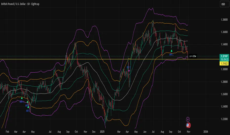
Z-Score Bands + SignalsZ-Score Statistical Market Analyzer
A multi-dimensional market structure indicator based on standardized deviation & regime logic
English Description
Concept
This indicator builds a statistical model of price behaviour by converting every candle’s movement into a Z-score — how many standard deviations each close is away from its moving average.
It visualizes the normal distribution structure of returns and provides adaptive entry signals for both Mean Reversion and Breakout regimes.
Rather than predicting price direction, it measures statistical displacement from equilibrium and dynamically adjusts the decision logic according to the market’s volatility regime.
⚙️ Main Components
Z-Score Bands (±1σ, ±2σ, ±3σ)
– The core structure visualizes volatility boundaries based on rolling mean and standard deviation.
– Price outside ±2σ often indicates statistical extremes.
Dual Signal Systems
Mean Reversion (MRL / MRS): when price (or return z-score) crosses back inside ±2σ bands.
Breakout (BOL / BOS): when price continues to expand beyond ±2σ.
Volatility Regime Classification
The indicator detects whether the market is currently in a low-vol or high-vol regime using percentile statistics of σ.
Low vol → Mean Reversion preferred
High vol → Breakout preferred
🧠 Adaptive Switches
A. Freeze MA/σ - Use previous-bar stats to avoid repainting and lag.
B. Confirm on Close - Only generate signals once the base-timeframe bar closes (eliminates look-ahead bias).
C. Return-based Signal - Use log-return Z-score instead of price deviation — normalizes volatility across assets.
D. Outlier Filter - Exclude bars with abnormal single-bar returns (e.g., >20%). Reduces false spikes.
E. Regime Gating - Automatically switch between Mean Reversion and Breakout logic depending on volatility percentile.
Each module can be toggled individually to test different statistical behaviours or tailor to a specific market condition.
📊 Interpretation
When the histogram of returns approximates a normal distribution, mean-reversion logic is often more effective.
When price persistently drifts beyond ±2σ or ±3σ, the distribution becomes leptokurtic (fat-tailed) — a breakout structure dominates.
Hence, this tool can help you:
Identify whether an asset behaves more “Gaussian” or “fat-tailed”;
Select the correct trading regime (MR or BO);
Quantitatively measure market tension and volatility clusters.
🧩 Recommended Use
Works on any timeframe and any asset.
Best used on liquid instruments (e.g., XAU/USD, indices, major FX pairs).
Combine with volume, sentiment or structural filters to confirm signals.
For strategy automation, pair with the companion script:
🧠 “Z-Score Strategy • Multi-Source Confirm (MRL/MRS/BOL/BOS)”.
⚠️ Disclaimer
This script is designed for educational and research purposes.
Statistical deviation ≠ directional prediction — use with sound risk management.
Past distribution patterns may shift under new volatility regimes.
==================================================================================
中文说明(简体)
概念简介
该指标基于价格的统计分布原理,将每根 K 线的波动转化为标准化的 Z-Score(标准差偏离值),用于刻画市场处于均衡或偏离状态。
它同时支持 均值回归(Mean Reversion) 与 突破延展(Breakout) 两种逻辑,并可根据市场波动结构自动切换策略模式。
⚙️ 主要功能模块
Z-Score 通道(±1σ / ±2σ / ±3σ)
用滚动均值与标准差动态绘制的统计波动带,价格超出 ±2σ 区域通常意味着极端偏离。
双信号系统
MRL / MRS(均值回归多空):价格重新回到 ±2σ 以内时触发。
BOL / BOS(突破延展多空):价格持续运行在 ±2σ 之外时触发。
波动率分层
自动识别市场处于高波动还是低波动区间:
低波动期 → 适合均值回归逻辑;
高波动期 → 适合突破趋势逻辑。
🧠 A–E 模块说明
A. 固定统计参数:使用上一根 K 线的均值和标准差,防止重绘。
B. 收盘确认信号:仅在当前时间框架收盘后生成信号,避免前视偏差。
C. 收益率信号模式:采用对数收益率的 Z-Score,更具普适性。
D. 异常波过滤:忽略单根极端波动(如 >20%)的噪声信号。
E. 波动率调节逻辑:根据市场处于高/低波动区间,自动切换 MRL/MRS 或 BOL/BOS。
📊 应用解读
如果收益率分布接近正态分布 → 市场倾向震荡,MRL/MRS 效果较佳;
若价格频繁偏离 ±2σ 或 ±3σ → 市场呈现“肥尾”分布,趋势延展占主导。
因此,该指标的核心目标是:
识别当前市场的统计结构类型;
根据波动特征自动切换交易逻辑;
提供结构化、可量化的市场状态刻画。
💡 使用建议
适用于所有时间框架与金融品种。
建议结合成交量或结构性指标过滤。
若用于策略回测,可搭配同名 “Z-Score Strategy • Multi-Source Confirm” 策略脚本。
⚠️ 免责声明
本指标仅用于研究与教学,不构成任何投资建议。
统计偏离 ≠ 趋势预测,实际市场行为可能在不同波动结构下改变。
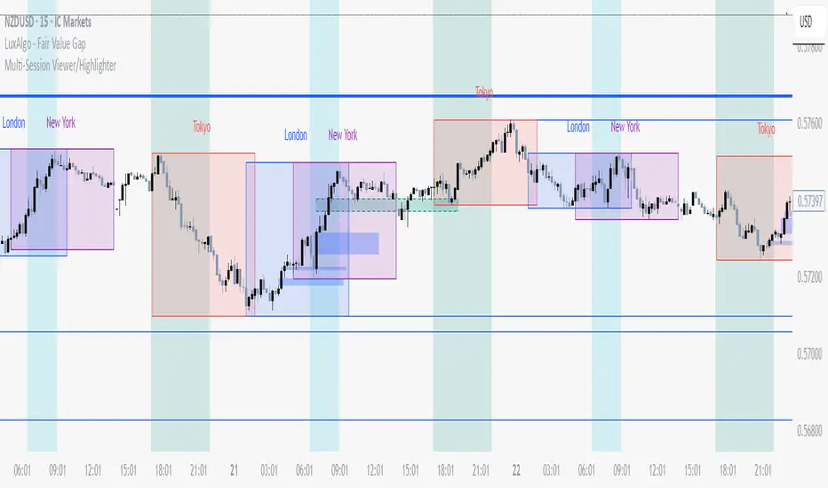
Multi-Session Viewer and AnalyzerFully customizable multi-session viewer that takes session analysis to the next level. It allows you to fully customize each session to your liking. Includes a feature that highlights certain periods of time on the chart and a Time Range Marker.
It helps you analyze the instrument that you trade and pinpoint which times are more volatile than others. It also helps you choose the best time to trade your instrument and align your life schedule with the market.
NZDUSD Example:
- 3 major sessions displayed.
- Although this is NZDUSD, Sydney is not the best time to trade this pair. Volatility picks up at Tokyo open.
- I have time to trade in the evening from 18:00 to 22:00 PST. I live in a different time zone, whereas market is based on EST. How does the pair behave during the time I am available to trade based on my time zone? Time Range Marker feature allows you to see this clearly on the chart (black lines).
- I have some time in the morning to trade during New York session, but there is no way I am waking up at 05:00 PST. 06:30 PST seems doable. Blue highlighted area is good time to trade during New York session based on what Bob said. It seem like this aligns with when I am available and when I am able to trade. Volatility is also at its peak.
- I am also available to trade between London close and Tokyo open on some days of the week, but... based on what I see, green highlighted area is clearly showing that I probably don't want to waste my time trading this pair from London close and until Tokyo open. I will use this time for something else rather than be stuck in a range.
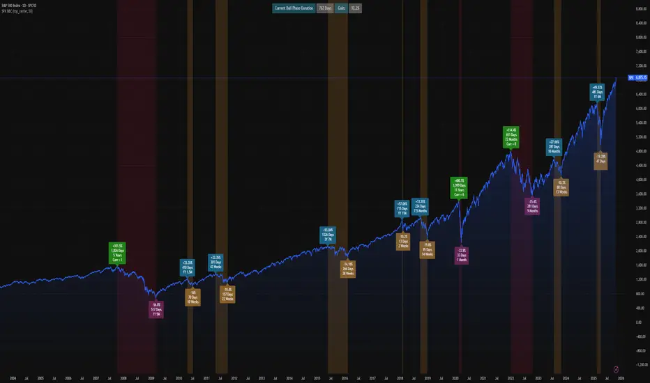
SPX Bull Market, Bear market and Corrections Since 1929 This script show visually with labels all the BULL & BEAR Market since 1929 with intermediary corrections.
Bear Market = Price drop of >=20% (based on closing price not intra day low)
Corrections = Price drop of >=10% and < 20% (based on closing price not intra day low, in intraday price it may go beyond 20% but closes in less than 20% )
The script doesn't update as we move forward , I need to manually update during every correction/bull/bear phases.
It is a good visual to study the past bull and bear market to gain some key insights!

Proactive Breakout Predictor - SAINTThe Proactive Breakout Predictor+ is an advanced intraday trading indicator designed to detect and confirm breakout opportunities with high accuracy — before they fully develop, and to identify ideal retest entries after the initial breakout.
It combines multiple layers of market structure, momentum, trend, and volume analysis to eliminate false breakouts and help traders enter with confidence.
Signal Type | Chart Marker | Meaning Bullish Breakout | 🟢 Up Triangle | Confirmed bullish breakout — strong upward
momentum with volume and trend confirmation.
Bearish Breakout | 🔴 Down Triangle | Confirmed bearish breakout — strong downward
momentum with volume and trend confirmation.
Bullish Retest | 🟢 Small Green Circle | Price retests breakout zone with low volume —
ideal re-entry or add-on for longs.
Bearish Retest | 🔴 Small Red Circle | Price retests breakdown zone with low volume —
ideal re-entry or add-on for shorts.

Algoritmictrader2025 ALGO System profitability works with a minimum profit margin of 75% and the maximum profit margin per share is around 95%. The software costs $150 per month.

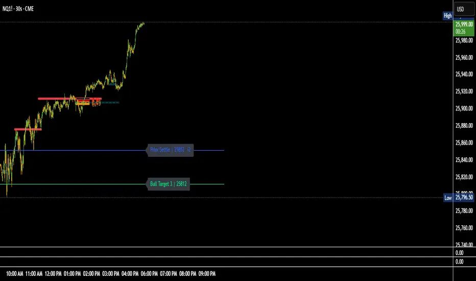
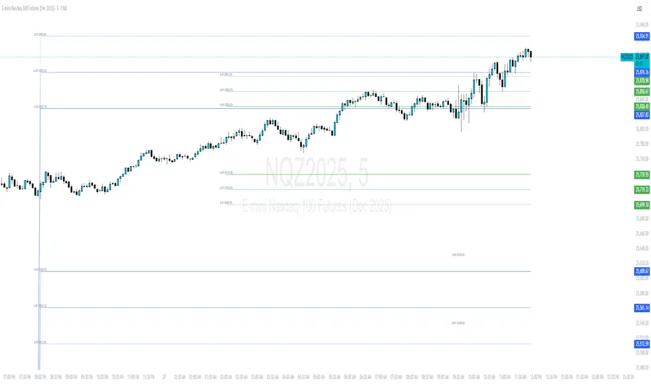
NQ Key Levels MapThe NQ Key Levels Map is a fully customizable tool designed to visually mark your most important trading levels on the Nasdaq futures (NQ) chart. It provides quick at-a-glance reference points for both bullish and bearish scenarios, as well as key overnight and contextual levels — all color-coded, labeled, and positioned exactly how you prefer.
This indicator helps traders maintain spatial awareness of critical price zones throughout the session without cluttering the chart.
💡 Key Features:
🟩 Bullish Levels (Green)
Max ATM – highest key level or equilibrium pivot.
Bull Trigger – upside breakout or entry confirmation.
Bull Targets 1–3 – progressive profit targets for bullish continuation.
🟥 Bearish Levels (Red)
Min ATM – lowest key level or equilibrium pivot.
Bear Trigger – downside breakout or short confirmation.
Bear Targets 1–3 – progressive downside objectives.
Overnight Low – prior session low reference.
🟦 Contextual Levels (Blue)
Overnight High – prior session high reference.
Flip Area – inflection zone where sentiment can shift.
Prior Settle – yesterday’s settlement price anchor.
Session 30 Second OR DeviationsThis indicator will plot the -4, -6, and -8 levels in color coded fashion based on session. We look for price reactions at these levels. It will plot the Asia session first 30 second candle, same with London, and New York.
BTC Open interest (binance, bybit, okx, bitget, htx, deribit)📈 BTC Open Interest Candles (Binance, Bybit, OKX, Bitget, HTX, Deribit)
🌟 Overview
This Pine Script indicator fetches real-time Bitcoin (BTC) perpetual futures open interest (OI) data from major cryptocurrency exchanges (Binance, OKX, Bybit, Bitget, HTX, Deribit), aggregates it, and visualizes it as candlesticks on the chart. Each candlestick represents the combined OI values at the open, high, low, and close of that bar. Candlestick colors change based on whether the current bar’s close OI is higher or lower than the previous bar’s, allowing intuitive tracking of OI fluctuations.
✨ Key Features
Multi-exchange OI aggregation: Combines OI data from selected exchanges to create a unified OI candlestick series.
Candlestick visualization: Converts aggregated OI values into open, high, low, and close values to plot candlestick charts, clearly showing the range and trend of OI over time.
Color-coded OI change:
Close OI higher than previous bar → teal candlestick (OI increase)
Close OI lower than previous bar → red candlestick (OI decrease)
⚙️ Inputs
Show Binance true Include Binance OI in the aggregation.
Show OKX true Include OKX OI in the aggregation.
Show Bybit true Include Bybit OI in the aggregation.
Show Bitget true Include Bitget OI in the aggregation.
Show HTX true Include HTX OI in the aggregation.
Show Deribit true Include Deribit OI in the aggregation.
📊 Calculation Methodology
Requests OI open, high, low, close values for the specified exchange using request.security().
Missing data (na) is treated as 0 to prevent aggregation errors.
Returns OI values as arrays.
➕ Aggregation of individual OI
Variables combinedOiOpen, combinedOiHigh, combinedOiLow, combinedOiClose initialized to 0.
Calls getOI for each enabled exchange and adds returned values to the combined variables.
🎨 Candlestick color determination
oiColorCond checks whether combinedOiClose > combinedOiClose .
True → openInterestColor = color.teal (OI increase)
False → openInterestColor = color.red (OI decrease)
🕯 Candlestick plotting
plotCandles ensures at least one exchange is selected.
plotcandle() is called with na values if no exchanges are selected to avoid drawing candles.
Candle body, wick, and border colors follow openInterestColor.
💡 How to Use
🌐 Integrated market sentiment
Observe overall market OI changes using a unified candlestick chart rather than fragmented exchange data to understand market sentiment and capital flow.
🔍 Compare with price movements
Analyze price charts alongside OI candlesticks to see how OI changes affect (or are affected by) price.
🟢 Price rising + teal OI candlestick (OI increase): Indicates bullish momentum from new long entries or short covering.
🔴 Price falling + red OI candlestick (OI decrease): Suggests bearish momentum from long liquidations or increased short covering.
📈 Price rising + red OI candlestick (OI decrease): Could reflect a short squeeze or profit-taking in long positions.
📉 Price falling + teal OI candlestick (OI increase): May indicate new short positions or forced long liquidations (stop-loss triggers).
⚡ Volatility prediction
Large OI candles or consecutive candles of a certain color can indicate imminent or ongoing significant market moves.

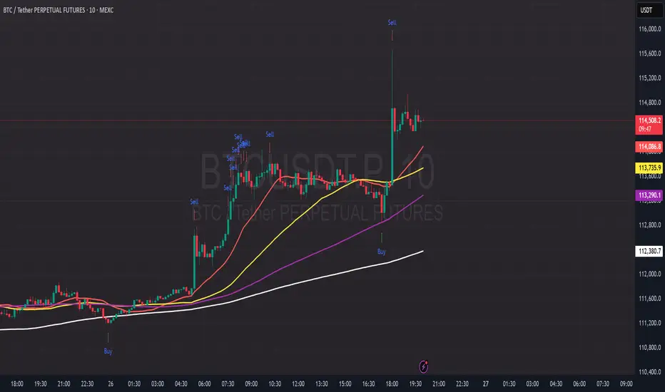
PDB - RSI Based Buy/Sell signals with 4 MARSI Based Buy/Sell Signals on Price chart + 4 MA System
This indicator plots RSI-based Buy & Sell signals directly on the price chart , combined with a 4-Moving-Average trend filter (20/50/100/200) for higher accuracy and cleaner trade timing.
The signal triggers when RSI reaches user-defined overbought/oversold levels, but unlike a standard RSI, this version plots the signals **on the chart**, not in the RSI window — making entries and exits easier to see in real time.
RSI Levels Are Fully Customizable
The default RSI thresholds are 30 (oversold) and 70 (overbought).
However, you can adjust these to fit your trading style. For example:
> When day trading on the 5–15 min timeframe, I personally use 35 (oversold) and 75 (overbought) to catch moves earlier.
> The example shown in the preview image uses 10-minute timeframe settings.
You can change the RSI levels to trigger signals from **any value you choose**, allowing you to tailor the indicator to scalping, day trading, or swing trading.
4 Moving Averages Included:
20, 50, 100, 200 MAs act as dynamic trend filters so you can:
✔ trade signals only in the direction of trend
✔ avoid false reversals
✔ identify momentum shifts more clearly
Works on all markets and timeframes — crypto, stocks, FX, indices.
PDB - RSI Buy & Sell Zones + SMA (PrintDemBandz)PDB - RSI Buy & Sell Zones
A clean, upgraded version of the RSI with shaded momentum zones to make entries and exits easier to spot. The background is divided into five color-coded zones so you instantly see when the market is shifting from bullish to bearish momentum.
Shaded Zones Explained:
| Zone | RSI Range | Zone Meaning |
| --------------------------- | --------- | ----------------------------------------------------- |
| Strong Buy (Dark Green) | < 30 | Oversold extreme – high probability bounce zone
| Buy Zone (Light Green) | 30–40 | Early accumulation & potential reversal area
| Neutral (Grey) | 40–60 | No edge zone – stay patient and wait for direction |
| Sell Zone (Light Red) | 60–70 | Market heating up – take profit or prepare to short |
| Strong Sell (Dark Red) | > 70 | Overbought extreme – high probability correction zone |
A dashed midline at 50 helps instantly gauge trend bias (above = bullish, below = bearish).
Use this RSI alone or combine with MACD or MA for stronger confirmations.
Search "PDB" in the indicators section for more free indicators.

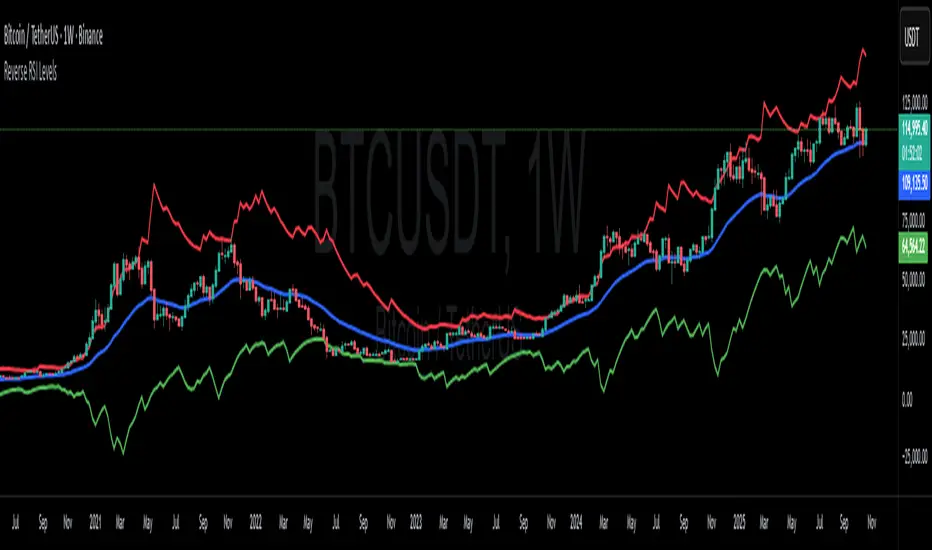
Reverse RSI LevelsSimple reverse RSI calculation
As default RSI values 30-50-70 are calculated into price.
This can be used similar to a bollinger band, but has also multiple other uses.
70 RSI works as overbought/resistance level.
50 RSI works as both support and resistance depending on the trend.
30 RSI works as oversold/support level.
Keep in mind that RSI levels can go extreme, specially in Crypto.
I haven't made it possible to adjust the default levels, but I've added 4 more calculations where you can plot reverse RSI calculations of your desired RSI values.
If you're a RSI geek, you probably use RSI quite often to see how high/low the RSI might go before finding a new support or resistance level. Now you can just put the RSI level into on of the 4 slots in the settings and see where that support/resistance level might be on the chart.
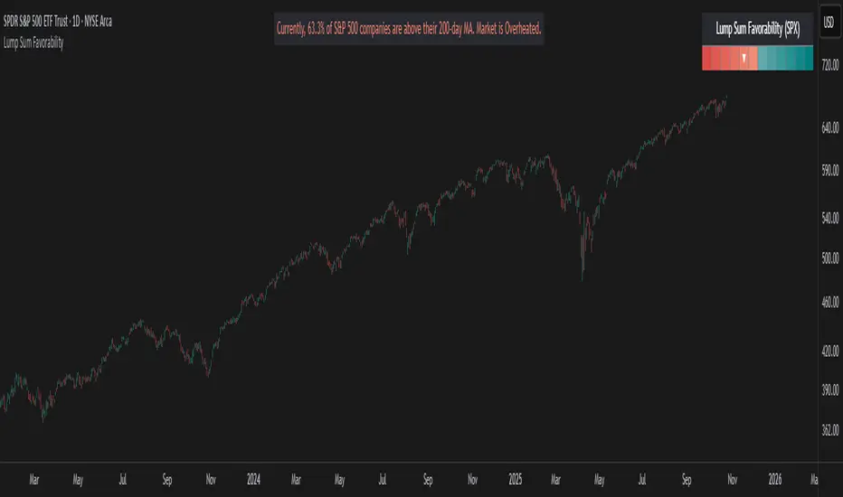
Lump Sum Favorability (SPX & NDX)This indicator provides a visual dashboard to gauge the statistical favorability of deploying a "Lump Sum" investment into the SPX (S&P 500) or NDX (Nasdaq 100).
The primary goal is not to time the exact market bottom, but to identify zones of significant pessimism or euphoria. Historically, periods of indiscriminate selling have represented high-probability entry points for long-term investors.
The dashboard consists of two parts:
1. The Favorability Gauge: A 12-segment gauge that moves from Red (Unfavorable) to Teal (Favorable).
2. The Summary Text: An optional text box (enabled in settings) that provides a plain-English summary of the current market breadth.
---
The Method: Market Breadth
This indicator is not based on the price of the index itself. Price-based indicators (like an RSI on the SPX) can be misleading. In a market-cap-weighted index, a few mega-cap stocks can hold the index price up while the vast majority of "average" stocks are already in a deep bear market.
This tool uses Market Breadth to measure the true, underlying health and participation of the entire market.
How It Works
1. Data Source: The indicator pulls the daily percentage of companies within the selected index (SPX or NDX) that are trading above their 200-day moving average. (Data tickers: S5TH for SPX, NDTH for NDX).
2. Smoothing: This raw data is volatile. To filter out daily noise and confirm a persistent trend, the indicator calculates a 5-day Simple Moving Average (SMA) of this percentage. This is the value used by the indicator.
3. Interpretation:
High Value (>= 50%): More than half of the stocks are above their long-term average. This signifies the market is "Overheated" or in a risk-on phase. The favorability for a new lump sum investment is considered Low.
Low Value (< 50%): Less than half of the stocks are above their long-term average. This signifies "Oversold" conditions or capitulation. These moments historically offer the best favorability for starting a new long-term investment.
---
How to Use the Indicator
1. The Favorability Gauge
The gauge is designed to be intuitive: Red means "Stop/Caution," and Teal means "Go/Opportunity."
Note: The gauge's logic is inverted from the data value to achieve this simplicity.
Red Zone (Left): UNFAVORABLE
This corresponds to a high percentage of stocks being above their 200d MA (>= 50%). The market is considered Overheated, and the favorability for a new lump sum investment is low.
Teal Zone (Right): FAVORABLE
This corresponds to a low percentage of stocks being above their 200d MA (< 50%). The market is considered Oversold, and the favorability for a new lump sum investment is high.
2. The Summary Text
When "Show Summary Text" is enabled in the settings, a box will appear at the top-center of your chart. This box provides a clear, data-driven summary, such as:
"Currently, only 22% of S&P 500 companies are above their 200-day MA. Market is Oversold."
The color of this text will automatically change to match the market state (Red for Overheated, Teal for Oversold), providing instant confirmation of the gauge's reading.
---
Settings
Market: Choose the index to analyze: SPX (S&P 500) or NDX (Nasdaq 100).
Gauge Position: Select where the gauge dashboard should appear on your chart (default is Bottom Right).
Show Summary Text: Toggle the descriptive text box on or off (default is On).
---
This indicator is a statistical and historical guide, not a financial advice or timing signal. It is designed to measure favorability based on past market behavior, not to provide certainty.
Extreme oversold conditions can persist, and markets can always go lower. This tool should be used as one component of a broader investment and risk-management framework. Past performance is not a guarantee of future results.
DAX Zonen Ergänzungen (Pro Signale + EMAs mit Filter RSI MACD)📊 DAX Zones Enhancements (Pro Signals + EMA with RSI & MACD Filter)
Description:
This indicator enhances DAX trading analysis by combining dynamic support/resistance zones with professional-level signal filters. It automatically detects potential buy and sell zones and confirms them using EMA trends, RSI conditions, and MACD momentum.
Key features:
🔹 Visual display of DAX high- and low-price zones
🔹 EMA-based trend confirmation
🔹 RSI and MACD filters to reduce false signals
🔹 Customizable alerts when price interacts with key zones
🔹 Works on multiple timeframes
Ideal for traders who want a clean, rule-based approach to identifying high-probability entries and exits on the DAX index.
