Custom ZigZag IndicatorOverview
The Custom ZigZag Indicator is a technical analysis tool built in Pine Script (version 5) for TradingView. It overlays on price charts to visualize market trends by connecting significant swing highs and lows, filtering out minor price noise. This helps identify the overall market direction (uptrends or downtrends), potential reversal points, and key support/resistance levels. Unlike standard price lines, it "zigzags" only between meaningful pivots, making trends clearer.
Core Logic and How It Works
The script uses a state-machine approach to track market direction and pivots:
Initialization
Starts assuming an upward trend on the first bar.
sets initial high/low prices and bar indices based on the current bar's high/low.
Direction Tracking:
Upward Trend (direction = 1):
Monitors for new highs: If the current high exceeds the tracked high, update the high price and bar.
Checks for reversal: If the low drops below the high by the deviation percentage (e.g., high * (1 - 0.05) for 5%), it signals a downtrend reversal.
Draws a green line from the last pivot (low) to the new high.
If labels are enabled, adds a label: "HH" (Higher High if above previous high), "LH" (Lower High if below), or "H" (for the first one).
Updates the last high and switches to downward direction.
Downward Trend (direction = -1):
Monitors for new lows: If the current low is below the tracked low, update the low price and bar.
Checks for reversal: If the high rises above the low by the deviation percentage (e.g., low * (1 + 0.05)), it signals an uptrend reversal.
Draws a red line from the last pivot (high) to the new low.
If labels are enabled, adds a label: "LL" (Lower Low if below previous low), "HL" (Higher Low if above), or "L" (for the first one).
Updates the last low and switches to upward direction.
חפש סקריפטים עבור "track"

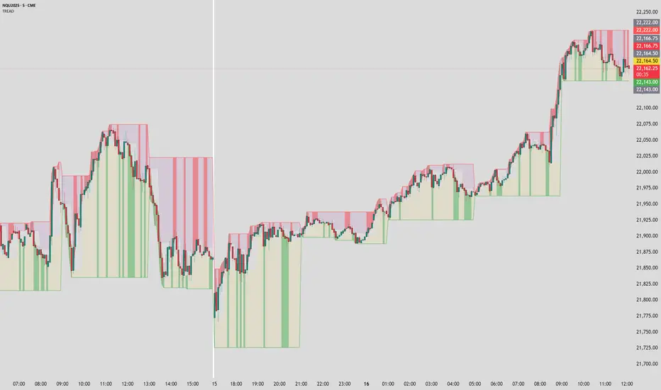
Timeframe Resistance Evaluation And Detection - CoffeeKillerTREAD - Timeframe Resistance Evaluation And Detection Guide
🔔 Important Technical Limitation 🔔
**This indicator does NOT fetch true higher timeframe data.** Instead, it simulates higher timeframe levels by aggregating data from your current chart timeframe. This means:
- Results will vary depending on what chart timeframe you're viewing
- Levels may not match actual higher timeframe candle highs/lows
- You might miss important wicks or gaps that occurred between chart timeframe bars
- **Always verify levels against actual higher timeframe charts before trading**
Welcome traders! This guide will walk you through the TREAD (Timeframe Resistance Evaluation And Detection) indicator, a multi-timeframe analysis tool developed by CoffeeKiller that identifies support and resistance confluence across different time periods.(I am 50+ year old trader and always thought I was bad a teaching and explaining so you get a AI guide. I personally use this on the 5 minute chart with the default settings, but to each there own and if you can improve the trend detection methods please DM me. I would like to see the code. Thanks)
Core Components
1. Dual Timeframe Level Tracking
- Short Timeframe Levels: Tracks opening price extremes within shorter periods
- Long Timeframe Levels: Tracks actual high/low extremes within longer periods
- Dynamic Reset Mechanism: Levels reset at the start of each new timeframe period
- Momentum Detection: Identifies when levels change mid-period, indicating active price movement
2. Visual Zone System
- High Zones: Areas between long timeframe highs and short timeframe highs
- Low Zones: Areas between long timeframe lows and short timeframe lows
- Fill Coloring: Dynamic colors based on whether levels are static or actively changing
- Momentum Highlighting: Special colors when levels break during active periods
3. Customizable Display Options
- Multiple Plot Styles: Line, circles, or cross markers
- Flexible Timeframe Selection: Wide range of short and long timeframe combinations
- Color Customization: Separate colors for each level type and momentum state
- Toggle Controls: Show/hide different elements based on trading preference
Main Features
Timeframe Settings
- Short Timeframe Options: 15m, 30m, 1h, 2h, 4h
- Long Timeframe Options: 1h, 2h, 4h, 8h, 12h, 1D, 1W
- Recommended Combinations:
- Scalping: 15m/1h or 30m/2h
- Day Trading: 30m/4h or 1h/4h
- Swing Trading: 4h/1D or 1D/1W
Display Configuration
- Level Visibility: Toggle short/long timeframe levels independently
- Fill Zone Control: Enable/disable colored zones between levels
- Momentum Fills: Special highlighting for actively changing levels
- Line Customization: Width, style, and color options for all elements
Color System
- Short TF High: Default red for resistance levels
- Short TF Low: Default green for support levels
- Long TF High: Transparent red for broader resistance context
- Long TF Low: Transparent green for broader support context
- Momentum Colors: Brighter colors when levels are actively changing
Technical Implementation Details
How Level Tracking Works
The indicator uses a custom tracking function that:
1. Detects Timeframe Periods: Uses `time()` function to identify when new periods begin
2. Tracks Extremes: Monitors highest/lowest values within each period
3. Resets on New Periods: Clears tracking when timeframe periods change
4. Updates Mid-Period: Continues tracking if new extremes are reached
The Timeframe Limitation Explained
`pinescript
// What the indicator does:
short_tf_start = ta.change(time(short_timeframe)) != 0 // Detects 30m period start
= track_highest(open, short_tf_start) // BUT uses chart TF opens!
// What true multi-timeframe would be:
// short_tf_high = request.security(syminfo.tickerid, short_timeframe, high)
`
This means:
- On a 5m chart with 30m/4h settings: Tracks 5m bar opens during 30m and 4h windows
- On a 1m chart with same settings: Tracks 1m bar opens during 30m and 4h windows
- Results will be different between chart timeframes
- May miss important price action that occurred between your chart's bars
Visual Elements
1. Level Lines
- Short TF High: Upper resistance line from shorter timeframe analysis
- Short TF Low: Lower support line from shorter timeframe analysis
- Long TF High: Broader resistance context from longer timeframe
- Long TF Low: Broader support context from longer timeframe
2. Zone Fills
- High Zone: Area between long TF high and short TF high (potential resistance cluster)
- Low Zone: Area between long TF low and short TF low (potential support cluster)
- Regular Fill: Standard transparency when levels are static
- Momentum Fill: Enhanced visibility when levels are actively changing
3. Dynamic Coloring
- Static Periods: Normal colors when levels haven't changed recently
- Active Periods: Momentum colors when levels are being tested/broken
- Confluence Zones: Different intensities based on timeframe alignment
Trading Applications
1. Support/Resistance Trading
- Entry Points: Trade bounces from zone boundaries
- Confluence Areas: Focus on areas where short and long TF levels cluster
- Zone Breaks: Enter on confirmed breaks through entire zones
- Multiple Timeframe Confirmation: Stronger signals when both timeframes align
2. Range Trading
- Zone Boundaries: Use fill zones as range extremes
- Mean Reversion: Trade back toward opposite zone when price reaches extremes
- Breakout Preparation: Watch for momentum color changes indicating potential breakouts
- Risk Management: Place stops outside the opposite zone
3. Trend Following
- Direction Bias: Trade in direction of zone breaks
- Pullback Entries: Enter on pullbacks to broken zones (now support/resistance)
- Momentum Confirmation: Use momentum coloring to confirm trend strength
- Multiple Timeframe Alignment: Strongest trends when both timeframes agree
4. Scalping Applications
- Quick Bounces: Trade rapid moves between zone boundaries
- Momentum Signals: Enter when momentum colors appear
- Short-Term Targets: Use opposite zone as profit target
- Tight Stops: Place stops just outside current zone
Optimization Guide
1. Timeframe Selection
For Different Trading Styles:
- Scalping: 15m/1h - Quick levels, frequent updates
- Day Trading: 30m/4h - Balanced view, good for intraday moves
- Swing Trading: 4h/1D - Longer-term perspective, fewer false signals
- Position Trading: 1D/1W - Major structural levels
2. Chart Timeframe Considerations
**Important**: Your chart timeframe affects results
- Lower Chart TF: More granular level tracking, but may be noisy
- Higher Chart TF: Smoother levels, but may miss important price action
- Recommended: Use chart timeframe 2-4x smaller than short indicator timeframe
3. Display Settings
- Busy Charts: Disable fills, show only key levels
- Clean Analysis: Enable all fills and momentum coloring
- Multi-Monitor Setup: Use different color schemes for easy identification
- Mobile Trading: Increase line width for visibility
Best Practices
1. Level Verification
- Always Cross-Check: Verify levels against actual higher timeframe charts
- Multiple Timeframes: Check 2-3 different chart timeframes for consistency
- Price Action Confirmation: Wait for candlestick confirmation at levels
- Volume Analysis: Combine with volume for stronger confirmation
2. Risk Management
- Stop Placement: Use zones rather than exact prices for stops
- Position Sizing: Reduce size when zones are narrow (higher risk)
- Multiple Targets: Scale out at different zone boundaries
- False Break Protection: Allow for minor zone penetrations
3. Signal Quality Assessment
- Momentum Colors: Higher probability when momentum coloring appears
- Zone Width: Wider zones often provide stronger support/resistance
- Historical Testing: Backtest on your preferred timeframe combinations
- Market Conditions: Adjust sensitivity based on volatility
Advanced Features
1. Momentum Detection System
The indicator tracks when levels change mid-period:
`pinescript
short_high_changed = short_high != short_high and not short_tf_start
`
This identifies:
- Active level testing
- Potential breakout situations
- Increased market volatility
- Trend acceleration points
2. Dynamic Color System
Complex conditional logic determines fill colors:
- Static Zones: Regular transparency for stable levels
- Active Zones: Enhanced colors for changing levels
- Mixed States: Different combinations based on user preferences
- Custom Overrides: User can prioritize certain color schemes
3. Zone Interaction Analysis
- Convergence: When short and long TF levels approach each other
- Divergence: When timeframes show conflicting levels
- Alignment: When both timeframes agree on direction
- Transition: When one timeframe changes while other remains static
Common Issues and Solutions
1. Inconsistent Levels
Problem: Levels look different on various chart timeframes
Solution: Always verify against actual higher timeframe charts
2. Missing Price Action
Problem: Important wicks or gaps not reflected in levels
Solution: Use chart timeframe closer to indicator's short timeframe setting
3. Too Many Signals
Problem: Excessive level changes and momentum alerts
Solution: Increase timeframe settings or reduce chart timeframe granularity
4. Lagging Signals
Problem: Levels seem to update too slowly
Solution: Decrease chart timeframe or use more sensitive timeframe combinations
Recommended Setups
Conservative Approach
- Timeframes: 4h/1D
- Chart: 1h
- Display: Show fills only, no momentum coloring
- Use: Swing trading, position management
Aggressive Approach
- Timeframes: 15m/1h
- Chart: 5m
- Display: All features enabled, momentum highlighting
- Use: Scalping, quick reversal trades
Balanced Approach
- Timeframes: 30m/4h
- Chart: 15m
- Display: Selective fills, momentum on key levels
- Use: Day trading, multi-session analysis
Final Notes
**Remember**: This indicator provides a synthetic view of multi-timeframe levels, not true higher timeframe data. While useful for identifying potential confluence areas, always verify important levels by checking actual higher timeframe charts.
**Best Results When**:
- Combined with actual multi-timeframe analysis
- Used for confluence confirmation rather than primary signals
- Applied with proper risk management
- Verified against price action and volume
**DISCLAIMER**: This indicator and its signals are intended solely for educational and informational purposes. The timeframe limitation means results may not reflect true higher timeframe levels. Always conduct your own analysis and verify levels independently before making trading decisions. Trading involves significant risk of loss.
Inverse Fair Value Gap [Pro+]Introduction
Inverse Fair Value Gap° is a fully customizable charting tool built to track inversion fair value gap logic that occur after displacement events—specifically when Fair Value Gaps (FVGs) are closed through, and effectively flipping their original state. The tool is inspired by Inner Circle Trader (ICT) concepts, offering a clean visual interface to support traders studying price behaviour after liquidity sweeps, FVG closures, and highlighting mechanical swings targets.
This indicator does not draw zones or suggest direction. It operates entirely on confirmed price events and produces logic-bound visuals designed for traders who already understand IFVG-based reasoning and seek visual consistency across sessions, Timeframe on any instrument.
Key Terms and Definitions
Swing High / Swing Low: A swing high is a local price peak with lower highs on either side. A swing low is a local trough with higher lows on either side. These are used to detect where liquidity may rest and are required for confirming the initial raid condition in the IFVG model.
Liquidity Raid: This occurs when price trades through a prior swing high or low, effectively “sweeping” a level where orders may be clustered around. The raid is a required precursor to inversion logic in this model. The tool will not evaluate a potential Fair Value Gap or Inversion Fair Value Gap unless a swing high or low has been taken first.
Fair Value Gap (FVG): A Fair Value Gap is a price imbalance that occurs when a strong move leaves a gap between candles—specifically, when the high of one candle and the low of a later candle do not overlap. FVGs often emerge during displacement and are commonly studied as inefficiencies within a price leg.
Inversion Fair Value Gap: An inversion happens when price fully closes through an existing Fair Value Gap that raided liquidity, suggesting the original imbalance rebalanced, and looks to reverse its original role. For example, when a bearish FVG is closed above after raiding a swing low, it may present a shift in orderflow (bullish inversion). The tool recognizes IFVGs as “inverted” after a candle body candle closes through the gap post raid.
Displacement: A strong directional price move, typically with momentum, that leaves a Fair Value Gap behind. Displacement is important in inversion logic, as it creates the context and confidence in comparing and contrasting FVGs and Inversions for obvious flips in market behaviour.
IFVG Line: Once inversion occurs, the indicator draws a single horizontal array on the candle's close. It marks the start of model activation. This is not a prediction level or a support/resistance area, as it merely serves as a reference for when model logic is sequentially active.
Opposing Swing: The swing high or low opposite the one that was swept during the initial raid. This becomes the model’s first target for mechanical delivery and is automatically drawn once the IFVG line is plotted. When price reaches this swing, the model has reached its mechanical objective and could offer opportunities for further continuation to additional liquidity pools if orderflow continues to be present.
Invalidation: The Inversion Fair Value Gap is considered invalid in one of two scenarios, which the user can toggle individually: a body print back above/below the inversion in bearish/bullish conditions, or trading above/below the most recent swing high/low after the liquidity raid. The IFVG line will continue extending until the setup is invalidated by the chosen toggle, or when the Opposing Swing is reached.
Consequent Encroachment (CE): The midpoint (50%) of the FVG or IFVG. This line can be optionally displayed for users who use the midpoint of imbalances for reference of imbalance respect. It is not required by the model’s internal logic but may assist with discretionary interpretation.
Description
At its core, IFVG° follows a structured three-step logic sequence: a FVG is created, liquidity is taken, and the Fair Value Gap (FVG) inside of the leg of the raid is closed through, signally a potential orderflow shift. Once inversion is confirmed, an IFVG line is plotted at the close of the candle that caused the inversion, making it the structural anchor for the model.
The tool does not account for partial fills or candle wicks for FVGs or IFVGs. Only full-body closures through a qualifying FVG are recognized. When this occurs, a bullish or bearish inversion is plotted and the model becomes active. From there, the opposing swing (the unswept high or low from the displacement leg) is automatically drawn as the target for the model.
The model remains active until either the opposing swing is tagged (completion) or Invalidation Condition is triggered (close through IFVG, or price violating the liquidity raid swing). Upon invalidation, the IFVG line turns gray, signaling that the structure is no longer valid for ongoing tracking.
Key Features
The Bias allows traders to define whether to track bullish inversions (closing above bearish FVGs), bearish inversions (closing below bullish FVGs), or neutral to see both. This allows isolated directional focus as well as the ability to display all models.
The Liquidity Timeframe defines the Timeframe for swing highs and lows that are identified for the required liquidity raid. The Chart mode allows analysts to use the active chart Timeframe. Auto enables a pre-defined Timeframe Alignment, explained inside of the setting tooltip. Custom allows for user-defined Timeframe alignment, which is helpful when syncing with specific higher-Timeframe structures. Session allows the user to use session highs and lows for the liquidity raid. Observe the difference in the IFVG' model activations based on different Liquidity Timeframe configurations:
Chart:
Automatic:
Custom (4H):
Session:
The FVG Filter Timeframe requires the IFVG setup to trade into a FVG before qualifying the raid filter. For instance, setting this to 4H ensures that only setups that form within a 4-hour FVG. This gives analysts an additional filter to qualify the start of the mechanical model.
The Session Filter enables traders to define up to four specific Time blocks when the model is permitted to trigger. The Macros Only toggle filters setups further by limiting activation to the first and last 10 minutes of each hour, a filter inspired for intraday traders and scalpers.
The Invalidation Condition determines when a IFVG is considered no longer valid. The Close option will maintain the inversion as active until price prints a body past the IFVG. Swing will maintain the inversion as active until the most recent swing from the liquidity raid is traded through; in this case a warning icon will appear once price prints a candle body past the IFVG.
Model Style includes customizable controls for the IFVG line, the opposing swing marker, and invalidated states. Label appearance, line styles, and extension behaviour are fully user-controlled. Traders can also enable the Consequent Encroachment (CE) line, which marks the 50% midpoint of the FVG.
An Info Table is available to display the charts Timeframe, current model state, toggled bias, active Timeframes, asset, and Time filter. Its position is fully customizable and can be moved to match chart preferences.
How Traders Can Use the Indicator Effectively
IFVG° is not meant to identify trade signals, entries, or exits. It is best used as a visual tracker and confluence for structure-based delivery. The tool excels as a companion for:
Journaling and reviewing IFVG-based setups across Timeframes and sessions
Studying structural completion or invalidation behaviour
Tracking delayed deliveries and retracement-based logic
Traders using the tool should be familiar with FVG formations, inversion criterias, and the importance of orderflow once an opposing swing is reached.
Usage Guidance
Add the IFVG° to a TradingView chart. This is a fractal script and can be applied across any Timeframe or asset pairing.
Use the IFVG line to track inversion structure, monitor when inversions are created and negated, and reference the opposing swing to determine whether structural delivery has completed.
Use the IFVG in combination with your own discretion and narrative to assess when the model has flipped, held, or broken.
Terms and Conditions
Our charting tools are products provided for informational and educational purposes only and do not constitute financial, investment, or trading advice. Our charting tools are not designed to predict market movements or provide specific recommendations. Users should be aware that past performance is not indicative of future results and should not be relied upon for making financial decisions. By using our charting tools, the purchaser agrees that the seller and the creator are not responsible for any decisions made based on the information provided by these charting tools. The purchaser assumes full responsibility and liability for any actions taken and the consequences thereof, including any loss of money or investments that may occur as a result of using these products. Hence, by purchasing these charting tools, the customer accepts and acknowledges that the seller and the creator are not liable nor responsible for any unwanted outcome that arises from the development, the sale, or the use of these products. Finally, the purchaser indemnifies the seller from any and all liability. If the purchaser was invited through the Friends and Family Program, they acknowledge that the provided discount code only applies to the first initial purchase of any Toodegrees product. The purchaser is therefore responsible for cancelling – or requesting to cancel – their subscription in the event that they do not wish to continue using the product at full retail price. If the purchaser no longer wishes to use the products, they must unsubscribe from the membership service, if applicable. We hold no reimbursement, refund, or chargeback policy. Once these Terms and Conditions are accepted by the Customer, before purchase, no reimbursements, refunds or chargebacks will be provided under any circumstances.
By continuing to use these charting tools, the user acknowledges and agrees to the Terms and Conditions outlined in this legal disclaimer.
סקריפט בתשלום

TradeTrackerLibrary "TradeTracker"
Simple Library for tracking trades
method track(this)
tracks trade when called on every bar
Namespace types: Trade
Parameters:
this (Trade) : Trade object
Returns: current Trade object
Trade
Has the constituents to track trades generated by any method.
Fields:
id (series int)
direction (series int) : Trade direction. Positive values for long and negative values for short trades
initialEntry (series float) : Initial entry price. This value will not change even if the entry is changed in the lifecycle of the trade
entry (series float) : Updated entry price. Allows variations to initial calculated entry. Useful in cases of trailing entry.
initialStop (series float) : Initial stop. Similar to initial entry, this is the first calculated stop for the lifecycle of trade.
stop (series float) : Trailing Stop. If there is no trailing, the value will be same as that of initial trade
targets (array) : array of target values.
startBar (series int) : bar index of starting bar. Set by default when object is created. No need to alter this after that.
endBar (series int) : bar index of last bar in trade. Set by tracker on each execution
startTime (series int) : time of the start bar. Set by default when object is created. No need to alter this after that.
endTime (series int) : time of the ending bar. Updated by tracking method.
status (series int) : Integer parameter to track the status of the trade
retest (series bool) : Boolean parameter to notify if there was retest of the entry price
BUY & SELL Dynamic DCA StrategyOverview
The BUY & SELL Dynamic DCA Strategy is a versatile Pine Script indicator designed for traders seeking a robust Dollar Cost Averaging (DCA) approach to manage both long and short positions across various market conditions and timeframes. This innovative tool combines breakout-based level initiation with a dynamic volatility adjustment, enabling traders to enter positions at optimal DCA points, average them strategically, and manage risk with adjustable stop-loss and take-profit levels. Ideal for scalping on short timeframes (1-minute, 5-minute) or swing trading on longer ones (15-minute, 1-hour, 4-hour).
Purpose and Originality
The "BUY & SELL Dynamic DCA Strategy" stands out by integrating several trading concepts into a cohesive, trader-friendly system. While it leverages familiar elements like breakout points and ATR (Average True Range), its originality lies in:
Dynamic Volatility Adjustment: A custom volatility factor, derived from a capped ATR calculation, dynamically scales DCA entry, averaging, and stop-loss levels. This ensures the strategy adapts to market conditions, tightening in low volatility for scalping and widening in high volatility for swing trading.
Dual-Direction DCA: Supports both buy (long) entries on pullbacks and sell (short) entries on rallies, with tailored averaging and exit strategies for each.
Timeframe Versatility: Adjusts its sensitivity based on the chart timeframe, making it suitable for rapid scalping or longer-term trend riding without requiring manual recalibration.
This unique synthesis justifies its publication as a invite-only script, offering a practical tool that enhances traditional DCA methods with adaptive precision.
How It Works
The indicator operates through a multi-step process designed to optimize entry, averaging, and exit points:
1. Initial Level Setting:
Utilizes high and low threshold (calculated over a user-defined period) to establish initial DCA entry levels. If no threshold is detected, it defaults to the previous bar’s price, ensuring immediate applicability.
2. Dynamic DCA Entry:
Entry levels are adjusted using a proprietary volatility factor, which scales the distance from the current price. Long entries trigger when the price falls below this level, while short entries trigger when the price rises above it, with a volume confirmation filter to reduce noise.
3. Averaging Mechanism:
A secondary level (Averaging Level) allows traders to add to their position when the price moves further against the trade (down for longs, up for shorts). This level is also volatility-adjusted, providing a structured cost-reduction strategy.
4. Risk and Reward Management:
A Final Stop-Loss (Final SL) is set farther out, calculated as a multiple of the volatility-adjusted risk distance, offering protection after averaging.
Take-Profit (TP) levels are determined using a user-defined risk-to-reward ratio, ensuring a balanced exit strategy tailored to market movement.
5. Performance Tracking:
A real-time win/loss table in the top-right corner records trade outcomes, with wins and losses color-coded based on the trade direction (green/red for long, red/green for short), aiding performance evaluation.
Features
1. Dual-Mode Operation : Facilitates both long entries on price dips and short entries on price surges, adaptable to bullish and bearish markets.
2. Volatility-Adaptive Levels: Employs a custom ATR-based adjustment to scale entry, averaging, and stop-loss levels, enhancing responsiveness across timeframes.
3. Visual Tools: Features dashed lines and labels for DCA Entry (green for long, red for short), Final SL (red), and TP (cyan), with debug labels for entries and averages.
4. Timeframe Flexibility: Automatically adjusts threshold periods and volatility factors based on the chart timeframe (1m, 5m, 15m, 1h, 4h), optimizing for scalping or swing trading.
5. Customizable Parameters: Allows fine-tuning of period, DCA factors, and visibility options.
Settings
Base Length (default: 10): Base period for pivot calculations, scaled by timeframe (e.g., 10 becomes 20 on 5m).
Type: 'Wicks' (high/low) or 'Body' (open/close) for price-based levels.
RR Ratio (default: 1.2): Risk-to-reward ratio for TP calculation.
DCA Entry Factor (default: 1.0): Multiplier for volatility-adjusted DCA entry distance.
Avg Level Factor (default: 2.0): Multiplier for averaging level distance.
Final SL Factor (default: 3.0): Multiplier for final stop-loss distance.
SL Type: 'Close' or 'High/Low' for stop-loss evaluation.
Show DCA Entry, Show Avg Level, Show Final SL: Toggle visibility of respective lines.
Show Win/Loss Table: Enable/disable performance tracking.
Line Style: Select 'Solid', 'Dashed', or 'Dotted'.
Usage Instructions
1. Application:
Add the "BUY & SELL Dynamic DCA Strategy - JOAT" via the Pine Editor or community scripts on TradingView.
2. Configuration:
Scalping (1m, 5m): Set Base Length to 5-10, use a low DCA Entry Factor (0.5-1.0) for tight entries, and a Final SL Factor of 2.0-3.0.
Swing Trading (15m, 1h, 4h): Increase Base Length to 15-20, use a higher DCA Entry Factor (1.0-2.0), and set Final SL Factor to 3.0-4.0 for wider stops.
Enable visual elements and adjust Line Style as preferred.
3. Signal Interpretation:
Long Trade: A green dashed "DCA Entry" line below the price triggers a "Long Entry" label on crossover down.
Short Trade: A red dashed "DCA Entry" line above the price triggers a "Short Entry" label on crossover up.
Averaging: A yellow "Avg" label (long) or magenta "Avg" label (short) appears at the respective averaging level.
Exits: TP (cyan) for wins, Final SL (red) for losses, tracked in the win/loss table.
Trade Management:
Scalping: Use 1m/5m for quick trades, averaging as price moves against you.
Swing Trading: Use 15m/1h/4h to capture trends, averaging for cost adjustment.
Manually adjust position size for averaging based on risk tolerance.
5. Performance Monitoring:
The top-right table updates with wins (green/red) and losses (red/green) per trade type, helping assess strategy effectiveness.
Limitations
Manual Averaging: Requires manual position size adjustment at the Averaging Level; automation is not included.
Timeframe Sensitivity: May require parameter tuning for optimal performance across 1m to 4h.
No Trend Filter: Sideways markets may generate noise; adding a trend indicator could enhance accuracy (future development).
Initialization Delay: First trade may be delayed until a pivot is detected, using the current price as a fallback.
Originality Justification
The custom volAdj method, which caps ATR at a percentage of price and scales it by timeframe, offering a unique volatility adjustment not found in standard indicators.
The dual-direction DCA with averaging, combining long and short strategies with volatility-modulated levels, providing a comprehensive trading framework.
The timeframe-adaptive design, automatically adjusting pivot periods and volatility factors, making it a versatile tool across scalping and swing trading.

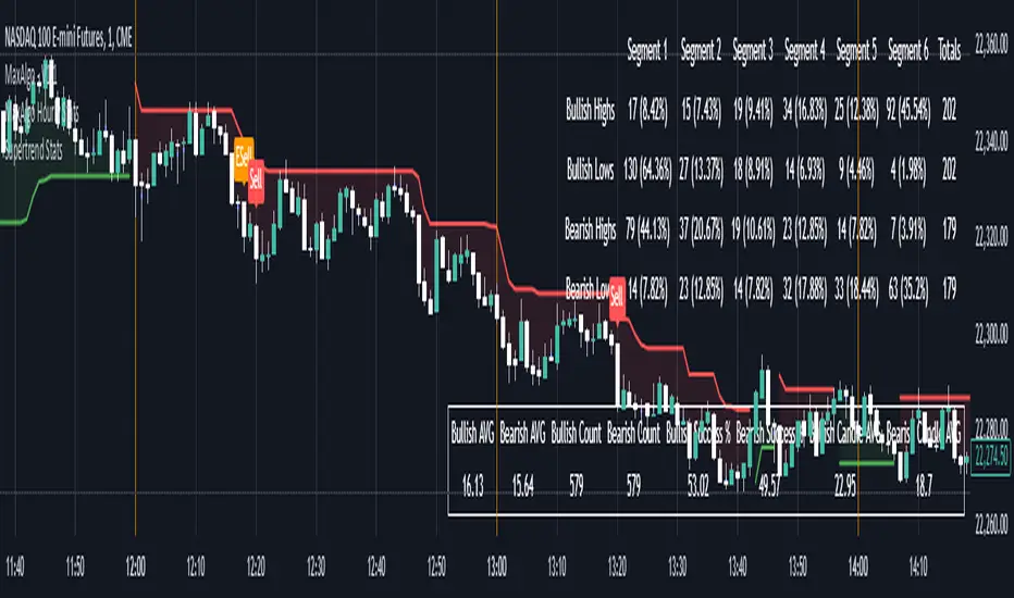
Supertrend StatsSupertrend with Probabilistic Stats and MA Filter
Overview: The Supertrend with Probabilistic Stats and MA Filter is a comprehensive TradingView Pine Script indicator designed to enhance trading strategies by combining the trend-detection capabilities of the Supertrend indicator with the trend-confirmation strength of Moving Averages (MA). Additionally, it offers robust statistical tracking to provide traders with valuable insights into the performance and reliability of their trading signals.
Key Features:
Supertrend Indicator Integration:
Trend Detection: Utilizes the Supertrend algorithm to identify prevailing market trends.
Buy/Sell Signals: Generates clear buy and sell signals based on trend reversals.
Customizable Parameters: Allows adjustment of ATR period and multiplier to suit different trading styles and market conditions.
Visual Aids: Plots Supertrend lines on the chart and highlights trend areas for easy visualization.
Moving Average (MA) Filter:
Trend Confirmation: Filters buy signals to occur only when the open price is above the MA and sell signals only when the open price is below the MA.
Customizable MA Types: Supports various MA types, including SMA, EMA, SMMA (RMA), WMA, and VWMA.
Flexible Configuration: Offers options to enable/disable the MA filter, select MA type, set MA length, and adjust MA source and offset.
Statistical Tracking:
Trimmed Mean Calculation: Computes trimmed means for bullish and bearish movements, removing outliers to provide a more accurate average movement.
Success Rate Metrics: Calculates the success rates (%) for both bullish and bearish signals, indicating the percentage of signals that resulted in favorable price movements.
Candle Count Analysis: Tracks the average number of candles each bullish and bearish move lasts, offering insights into the duration of trends.
Data Visualization: Presents all statistical data in a neatly formatted table on the chart, allowing for quick reference and analysis.
Customizable Statistics Table:
Text Color Customization: Provides an option to change the table text color to match personal preferences or chart aesthetics, enhancing readability.
Comprehensive Metrics: Displays key statistics such as Bullish/Bearish Averages, Counts, Success Rates, and Average Candle Counts.
Optional Pinbar Filtering:
Signal Refinement: Adds an additional layer of signal confirmation by filtering buy and sell signals based on pinbar candlestick patterns.
Adjustable Thresholds: Allows customization of the pinbar wick threshold to fine-tune signal accuracy.
Visual Enhancements:
Markers: Optionally displays markers on the first and last candles of bullish and bearish moves for better trend identification.
Highlighter: Shades the chart background to indicate current trend direction, aiding in visual trend recognition.
How It Works:
Trend Identification with Supertrend:
The indicator calculates the Supertrend based on user-defined ATR periods and multipliers.
It plots the Supertrend lines and generates buy/sell signals when the price crosses these lines, indicating a potential trend reversal.
Filtering Signals with Moving Average:
When the MA filter is enabled, the indicator ensures that buy signals are only considered valid if the candle's open price is above the selected MA, and sell signals only if the open price is below the MA.
This additional confirmation aligns trades with the broader market trend, potentially increasing signal reliability.
Statistical Analysis:
Upon triggering a buy or sell signal, the indicator records the entry price and tracks the subsequent price movements.
It calculates trimmed means to assess average movements while excluding extreme outliers.
Success rates are computed by comparing the closing price against the entry price, indicating how often signals result in favorable outcomes.
The average number of candles per move provides insight into trend duration and volatility.
Visualization and Customization:
All statistical data is presented in a table on the chart, with customizable text colors for enhanced readability.
Optional pinbar filtering and visual markers further refine and illustrate trading signals, aiding in decision-making.
Benefits to Traders:
Enhanced Signal Reliability:
By combining Supertrend with an MA filter, the indicator ensures that only signals aligning with the broader market trend are considered, potentially reducing false signals.
Data-Driven Decision Making:
The comprehensive statistical tracking offers traders insights into the performance of their signals, enabling informed adjustments to their trading strategies based on empirical data.
Trend Confirmation and Alignment:
The MA filter acts as a trend confirmation tool, ensuring that trades are placed in the direction of the prevailing trend, which can enhance the probability of successful trades.
Performance Metrics at a Glance:
The statistics table provides all necessary performance metrics in a single view, allowing traders to quickly assess the effectiveness of their strategy without sifting through extensive data.
Customization and Flexibility:
With options to adjust MA types, lengths, and table text colors, traders can tailor the indicator to fit their specific preferences and trading environments.
Visual Clarity and Aids:
The plotted Supertrend lines, MA line, signal markers, and highlighter enhance visual clarity, making it easier to identify trends and potential trade opportunities on the chart.
Usage Instructions:
Adding the Indicator:
Copy the Script: Select and copy the entire Pine Script provided.
Open TradingView: Navigate to TradingView and open your desired asset's chart.
Access Pine Editor: Click on the Pine Editor tab at the bottom of the TradingView interface.
Paste and Add to Chart: Paste the script into the editor and click "Add to Chart" to apply the indicator.
Configuring Settings:
Supertrend Parameters: Adjust the ATR period and multiplier to suit your trading style and the asset's volatility.
MA Filter Settings:
Enable MA Filter: Toggle "Enable MA Filter?" to ON to activate the filter.
Select MA Type: Choose from SMA, EMA, SMMA (RMA), WMA, or VWMA.
Set MA Length: Define the period for the MA calculation.
MA Source and Offset: Choose the price source (default is close) and set any desired plot offset.
Statistical Tracking:
Trimmed Mean Percentage: Set the percentage to trim outliers in mean calculations.
Show Cross Markers: Toggle to display or hide markers on the first and last candles of bullish and bearish moves.
Table Customization:
Table Text Color: Select your preferred text color for the statistics table to match your chart's theme or enhance readability.
Pinbar Filtering (Optional):
Enable Pinbar Filtering: Toggle to refine signals based on pinbar patterns.
Set Pinbar Wick Threshold: Adjust the threshold to define the characteristics of a valid pinbar.
Interpreting the Indicators:
Buy/Sell Signals: Look for labeled "BUY" and "SELL" signals on the chart that align with Supertrend reversals and MA conditions.
Statistics Table: Refer to the table located at the bottom right of the chart to assess:
Bullish/Bearish Averages: Average price movements following signals.
Counts: Total number of bullish and bearish signals.
Success Rates (%): Percentage of signals that resulted in profitable trades.
Candle Averages: Average duration of bullish and bearish moves in terms of candle counts.
Markers and Highlighter: Utilize visual markers and shaded trend areas to better understand market trends and the context of each signal.
Making Informed Decisions:
Assess Signal Performance: Use the success rates and averages to evaluate the effectiveness of your current settings and make necessary adjustments.
Adjust Parameters: Modify Supertrend and MA parameters based on observed performance and changing market conditions to optimize signal accuracy.
Combine with Other Analysis: Integrate insights from this indicator with other technical analysis tools and fundamental factors to form a holistic trading strategy.
Conclusion: The Supertrend with Probabilistic Stats and MA Filter indicator offers a powerful combination of trend detection, signal filtering, and statistical analysis. By providing detailed performance metrics and ensuring that trades align with the broader market trend, this indicator empowers traders to make more informed, data-driven decisions. Whether you're a novice seeking clarity or an experienced trader aiming to refine your strategy, this tool serves as a valuable asset in your trading toolkit.
If you have any further questions or require additional customizations, feel free to reach out!
PavanDeshetty-CallThe PavanDeshetty-Call indicator is a custom Pine Script tool designed to track options price movements for a specific call option and generate entry and exit signals based on predefined conditions. Below is a description of its key components:
Key Features:
Index Selection: Allows the user to select from major indices like NIFTY, BANKNIFTY, FINNIFTY, and MIDCPNIFTY. The selected index forms part of the option symbol.
Expiry Date Input: The user inputs the expiry day, month, and year, which helps to construct the full symbol for the call option being tracked.
Strike Price Selection: Allows the user to input a specific strike price for the call option, further refining the option symbol.
Option Symbol Generation: Based on the selected index, expiry date, and strike price, the indicator generates the symbol for the selected call option.
Data and Plotting:
Option Premium Data: The indicator fetches the open, high, low, and close data for the selected call option symbol using the request.security() function, which is then plotted as a candle chart. Green candles indicate price increases (close > open), while red candles indicate price decreases (close < open).
Entry and Exit Logic:
Entry Condition:
The indicator checks if the current option price is greater than or equal to 100.5% of the highest high of the previous "n" candles (the number of previous candles can be specified by the user).
If true, and if the user is not already in a position, a buy signal is generated.
Exit Condition:
The indicator checks if the option price has crossed below 99.5% of the previous candle's low.
If true, and if the user is in a position, a sell signal is generated.
Position Tracking:
The script uses a boolean variable in_position to track whether the user is currently in a trade. This prevents multiple entries and ensures that the exit condition resets the trade status.
Visual Signals:
Buy and Sell Signals:
Buy signals are plotted as green "Buy" labels at the bottom of the chart.
Sell signals are plotted as red "Sell" labels at the top of the chart.
After each signal, the flags for plotting the signals are reset.
Alerts:
Buy and Sell Alerts: The indicator includes alert conditions for both the buy and sell signals, allowing users to set up notifications when the entry or exit conditions are met.
This indicator is useful for traders looking to automate or track options trading based on specific strike prices and options expiry dates, combined with simple price-action-based entry and exit conditions.

Overbought / Oversold Screener## Introduction
**The Versatile RSI and Stochastic Multi-Symbol Screener**
**Unlock a wealth of trading opportunities with this customizable screener, designed to pinpoint potential overbought and oversold conditions across 17 symbols, with alert support!**
## Description
This screener is suitable for tracking multiple instruments continuously.
With the screener, you can see the instant RSI or Stochastic values of the instruments you are tracking, and easily catch the moments when they are overbought / oversold according to your settings.
The purpose of the screener is to facilitate the continuous tracking of multiple instruments. The user can track up to 17 different instruments in different time intervals. If they wish, they can set an alarm and learn overbought oversold according to the values they set for the time interval of the instruments they are tracking.**
Key Features:
Comprehensive Analysis:
Monitors RSI and Stochastic values for 17 symbols simultaneously.
Automatically includes the current chart's symbol for seamless integration.
Supports multiple timeframes to uncover trends across different time horizons.
Personalized Insights:
Adjust overbought and oversold thresholds to align with your trading strategy.
Sort results by symbol, RSI, or Stochastic values to prioritize your analysis.
Choose between Automatic, Dark, or Light mode for optimal viewing comfort.
Dynamic Visual Cues:
Instantly highlights oversold and overbought symbols based on threshold levels.
Timely Alerts:
Stay informed of potential trading opportunities with alerts for multiple oversold or overbought symbols.
## Settings
### Display
**Timeframe**
The screener displays the values according to the selected timeframe. The default timeframe is "Chart". For example, if the timeframe is set to "15m" here, the screener will show the RSI and stochastic values for the 15-minute chart.
** Theme **
This setting is for changing the theme of the screener. You can set the theme to "Automatic", "Dark", or "Light", with "Automatic" being the default value. When the "Automatic" theme is selected, the screener appearance will also be automatically updated when you enable or disable dark mode from the TradingView settings.
** Position **
This option is for setting the position of the table on the chart. The default setting is "middle right". The available options are (top, middle, bottom)-(left, center, right).
** Sort By **
This option is for changing the sorting order of the table. The default setting is "RSI Descending". The available options are (Symbol, RSI, Stoch)-(Ascending, Descending).
It is important to note that the overbought and oversold coloring of the symbols may also change when the sorting order is changed. If RSI is selected as the sorting order, the symbols will be colored according to the overbought and oversold threshold values specified for RSI. Similarly, if Stoch is selected as the sorting order, the symbols will be colored according to the overbought and oversold threshold values specified for Stoch.
From this perspective, you can also think of the sorting order as a change in the main indicator.
### RSI / Stochastic
This area is for selecting the parameters of the RSI and stochastic indicators. You can adjust the values for "length", "overbought", and "oversold" for both indicators according to your needs. The screener will perform all RSI and stochastic calculations according to these settings. All coloring in the table will also be according to the overbought and oversold values in these settings.
### Symbols
The symbols to be tracked in the table are selected from here. Up to 16 symbols can be selected from here. Since the symbol in the chart is automatically added to the table, there will always be at least 1 symbol in the table. Note that the symbol in the chart is shown in the table with "(C)". For example, if SPX is open in the chart, it is shown as SPX(C) in the table.
## Alerts
The screener is capable of notifying you with an alarm if multiple symbols are overbought or oversold according to the values you specify along with the desired timeframe. This way, you can instantly learn if multiple symbols are overbought or oversold with one alarm, saving you time.

True Gap Finder with Revisit DetectionTrue Gap Finder with Revisit Detection
This indicator is a powerful tool for intraday traders to identify and track price gaps. Unlike simple gap indicators, this script actively tracks the status of the gap, visualizing the void until it is filled (revisited) by price.
Key Features:
Active Gap Tracking: Finds gap-up and gap-down occurrences (where Low > Previous High or High < Previous Low) and actively tracks them.
Gap Zones (Clouds): Visually shades the empty "gap zone" (the void between the gap candles), making it instantly obvious where price needs to travel to fill the gap. The cloud disappears automatically once the gap is filled.
Dynamic Labels: automatically displays price labels at the origin of the gap, showing the specific price range (High-Low) that constitutes the gap. Labels are positioned intelligently to avoid cluttering current price action.
Alerts: Configurable alerts notify you the moment a gap is filled.
Customization: Full control over colors, clouds, labels, and alert settings to match your chart style.
How it works: The indicator tracks the most recent gap. If a new gap forms, it becomes the active focus. When price moves back to "close" or "fill" this gap area, the lines and clouds automatically stop plotting, giving you a clean chart that focuses only on open business.

Luxy Momentum, Trend, Bias and Breakout Indicators V7
TABLE OF CONTENTS
This is Version 7 (V7) - the latest and most optimized release. If you are using any older versions (V6, V5, V4, V3, etc.), it is highly recommended to replace them with V7.
Why This Indicator is Different
Who Should Use This
Core Components Overview
The UT Bot Trading System
Understanding the Market Bias Table
Candlestick Pattern Recognition
Visual Tools and Features
How to Use the Indicator
Performance and Optimization
FAQ
---
### CREDITS & ATTRIBUTION
This indicator implements proven trading concepts using entirely original code developed specifically for this project.
### CONCEPTUAL FOUNDATIONS
• UT Bot ATR Trailing System
- Original concept by @QuantNomad: (search "UT-Bot-Strategy"
- Our version is a complete reimplementation with significant enhancements:
- Volume-weighted momentum adjustment
- Composite stop loss from multiple S/R layers
- Multi-filter confirmation system (swing, %, 2-bar, ZLSMA)
- Full integration with multi-timeframe bias table
- Visual audit trail with freeze-on-touch
- NOTE: No code was copied - this is a complete reimplementation with enhancements.
• Standard Technical Indicators (Public Domain Formulas):
- Supertrend: ATR-based trend calculation with custom gradient fills
- MACD: Gerald Appel's formula with separation filters
- RSI: J. Welles Wilder's formula with pullback zone logic
- ADX/DMI: Custom trend strength formula inspired by Wilder's directional movement concept, reimplemented with volume weighting and efficiency metrics
- ZLSMA: Zero-lag formula enhanced with Hull MA and momentum prediction
### Custom Implementations
- Trend Strength: Inspired by Wilder's ADX concept but using volume-weighted pressure calculation and efficiency metrics (not traditional +DI/-DI smoothing)
- All code implementations are original
### ORIGINAL FEATURES (70%+ of codebase)
- Multi-Timeframe Bias Table with live updates
- Risk Management System (R-multiple TPs, freeze-on-touch)
- Opening Range Breakout tracker with session management
- Composite Stop Loss calculator using 6+ S/R layers
- Performance optimization system (caching, conditional calcs)
- VIX Fear Index integration
- Previous Day High/Low auto-detection
- Candlestick pattern recognition with interactive tooltips
- Smart label and visual management
- All UI/UX design and table architecture
### DEVELOPMENT PROCESS
**AI Assistance:** This indicator was developed over 2+ months with AI assistance (ChatGPT/Claude) used for:
- Writing Pine Script code based on design specifications
- Optimizing performance and fixing bugs
- Ensuring Pine Script v6 compliance
- Generating documentation
**Author's Role:** All trading concepts, system design, feature selection, integration logic, and strategic decisions are original work by the author. The AI was a coding tool, not the system designer.
**Transparency:** We believe in full disclosure - this project demonstrates how AI can be used as a powerful development tool while maintaining creative and strategic ownership.
---
1. WHY THIS INDICATOR IS DIFFERENT
Most traders use multiple separate indicators on their charts, leading to cluttered screens, conflicting signals, and analysis paralysis. The Suite solves this by integrating proven technical tools into a single, cohesive system.
Key Advantages:
All-in-One Design: Instead of loading 5-10 separate indicators, you get everything in one optimized script. This reduces chart clutter and improves TradingView performance.
Multi-Timeframe Bias Table: Unlike standard indicators that only show the current timeframe, the Bias Table aggregates trend signals across multiple timeframes simultaneously. See at a glance whether 1m, 5m, 15m, 1h are aligned bullish or bearish - no more switching between charts.
Smart Confirmations: The indicator doesn't just give signals - it shows you WHY. Every entry has multiple layers of confirmation (MA cross, MACD momentum, ADX strength, RSI pullback, volume, etc.) that you can toggle on/off.
Dynamic Stop Loss System: Instead of static ATR stops, the SL is calculated from multiple support/resistance layers: UT trailing line, Supertrend, VWAP, swing structure, and MA levels. This creates more intelligent, price-action-aware stops.
R-Multiple Take Profits: Built-in TP system calculates targets based on your initial risk (1R, 1.5R, 2R, 3R). Lines freeze when touched with visual checkmarks, giving you a clean audit trail of partial exits.
Educational Tooltips Everywhere: Every single input has detailed tooltips explaining what it does, typical values, and how it impacts trading. You're not guessing - you're learning as you configure.
Performance Optimized: Smart caching, conditional calculations, and modular design mean the indicator runs fast despite having 15+ features. Turn off what you don't use for even better performance.
No Repainting: All signals respect bar close. Alerts fire correctly. What you see in history is what you would have gotten in real-time.
What Makes It Unique:
Integrated UT Bot + Bias Table: No other indicator combines UT Bot's ATR trailing system with a live multi-timeframe dashboard. You get precision entries with macro trend context.
Candlestick Pattern Recognition with Interactive Tooltips: Patterns aren't just marked - hover over any emoji for a full explanation of what the pattern means and how to trade it.
Opening Range Breakout Tracker: Built-in ORB system for intraday traders with customizable session times and real-time status updates in the Bias Table.
Previous Day High/Low Auto-Detection: Automatically plots PDH/PDL on intraday charts with theme-aware colors. Updates daily without manual input.
Dynamic Row Labels in Bias Table: The table shows your actual settings (e.g., "EMA 10 > SMA 20") not generic labels. You know exactly what's being evaluated.
Modular Filter System: Instead of forcing a fixed methodology, the indicator lets you build your own strategy. Start with just UT Bot, add filters one at a time, test what works for your style.
---
2. WHO WHOULD USE THIS
Designed For:
Intermediate to Advanced Traders: You understand basic technical analysis (MAs, RSI, MACD) and want to combine multiple confirmations efficiently. This isn't a "one-click profit" system - it's a professional toolkit.
Multi-Timeframe Traders: If you trade one asset but check multiple timeframes for confirmation (e.g., enter on 5m after checking 15m and 1h alignment), the Bias Table will save you hours every week.
Trend Followers: The indicator excels at identifying and following trends using UT Bot, Supertrend, and MA systems. If you trade breakouts and pullbacks in trending markets, this is built for you.
Intraday and Swing Traders: Works equally well on 5m-1h charts (day trading) and 4h-D charts (swing trading). Scalpers can use it too with appropriate settings adjustments.
Discretionary Traders: This isn't a black-box system. You see all the components, understand the logic, and make final decisions. Perfect for traders who want tools, not automation.
Works Across All Markets:
Stocks (US, international)
Cryptocurrency (24/7 markets supported)
Forex pairs
Indices (SPY, QQQ, etc.)
Commodities
NOT Ideal For :
Complete Beginners: If you don't know what a moving average or RSI is, start with basics first. This indicator assumes foundational knowledge.
Algo Traders Seeking Black Box: This is discretionary. Signals require context and confirmation. Not suitable for blind automated execution.
Mean-Reversion Only Traders: The indicator is trend-following at its core. While VWAP bands support mean-reversion, the primary methodology is trend continuation.
---
3. CORE COMPONENTS OVERVIEW
The indicator combines these proven systems:
Trend Analysis:
Moving Averages: Four customizable MAs (Fast, Medium, Medium-Long, Long) with six types to choose from (EMA, SMA, WMA, VWMA, RMA, HMA). Mix and match for your style.
Supertrend: ATR-based trend indicator with unique gradient fill showing trend strength. One-sided ribbon visualization makes it easier to see momentum building or fading.
ZLSMA : Zero-lag linear-regression smoothed moving average. Reduces lag compared to traditional MAs while maintaining smooth curves.
Momentum & Filters:
MACD: Standard MACD with separation filter to avoid weak crossovers.
RSI: Pullback zone detection - only enter longs when RSI is in your defined "buy zone" and shorts in "sell zone".
ADX/DMI: Trend strength measurement with directional filter. Ensures you only trade when there's actual momentum.
Volume Filter: Relative volume confirmation - require above-average volume for entries.
Donchian Breakout: Optional channel breakout requirement.
Signal Systems:
UT Bot: The primary signal generator. ATR trailing stop that adapts to volatility and gives clear entry/exit points.
Base Signals: MA cross system with all the above filters applied. More conservative than UT Bot alone.
Market Bias Table: Multi-timeframe dashboard showing trend alignment across 7 timeframes plus macro bias (3-day, weekly, monthly, quarterly, VIX).
Candlestick Patterns: Six major reversal patterns auto-detected with interactive tooltips.
ORB Tracker: Opening range high/low with breakout status (intraday only).
PDH/PDL: Previous day levels plotted automatically on intraday charts.
VWAP + Bands : Session-anchored VWAP with up to three standard deviation band pairs.
---
4. THE UT BOT TRADING SYSTEM
The UT Bot is the heart of the indicator's signal generation. It's an advanced ATR trailing stop that adapts to market volatility.
Why UT Bot is Superior to Fixed Stops:
Traditional ATR stops use a fixed multiplier (e.g., "stop = entry - 2×ATR"). UT Bot is smarter:
It TRAILS the stop as price moves in your favor
It WIDENS during high volatility to avoid premature stops
It TIGHTENS during consolidation to lock in profits
It FLIPS when price breaks the trailing line, signaling reversals
Visual Elements You'll See:
Orange Trailing Line: The actual UT stop level that adapts bar-by-bar
Buy/Sell Labels: Aqua triangle (long) or orange triangle (short) when the line flips
ENTRY Line: Horizontal line at your entry price (optional, can be turned off)
Suggested Stop Loss: A composite SL calculated from multiple support/resistance layers:
- UT trailing line
- Supertrend level
- VWAP
- Swing structure (recent lows/highs)
- Long-term MA (200)
- ATR-based floor
Take Profit Lines: TP1, TP1.5, TP2, TP3 based on R-multiples. When price touches a TP, it's marked with a checkmark and the line freezes for audit trail purposes.
Status Messages: "SL Touched ❌" or "SL Frozen" when the trade leg completes.
How UT Bot Differs from Other ATR Systems:
Multiple Filters Available: You can require 2-bar confirmation, minimum % price change, swing structure alignment, or ZLSMA directional filter. Most UT implementations have none of these.
Smart SL Calculation: Instead of just using the UT line as your stop, the indicator suggests a better SL based on actual support/resistance. This prevents getting stopped out by wicks while keeping risk controlled.
Visual Audit Trail: All SL/TP lines freeze when touched with clear markers. You can review your trades weeks later and see exactly where entries, stops, and targets were.
Performance Options: "Draw UT visuals only on bar close" lets you reduce rendering load without affecting logic or alerts - critical for slower machines or 1m charts.
Trading Logic:
UT Bot flips direction (Buy or Sell signal appears)
Check Bias Table for multi-timeframe confirmation
Optional: Wait for Base signal or candlestick pattern
Enter at signal bar close or next bar open
Place stop at "Suggested Stop Loss" line
Scale out at TP levels (TP1, TP2, TP3)
Exit remaining position on opposite UT signal or stop hit
---
5. UNDERSTANDING THE MARKET BIAS TABLE
This is the indicator's unique multi-timeframe intelligence layer. Instead of looking at one chart at a time, the table aggregates signals across seven timeframes plus macro trend bias.
Why Multi-Timeframe Analysis Matters:
Professional traders check higher and lower timeframes for context:
Is the 1h uptrend aligning with my 5m entry?
Are all short-term timeframes bullish or just one?
Is the daily trend supportive or fighting me?
Doing this manually means opening multiple charts, checking each indicator, and making mental notes. The Bias Table does it automatically in one glance.
Table Structure:
Header Row:
On intraday charts: 1m, 5m, 15m, 30m, 1h, 2h, 4h (toggle which ones you want)
On daily+ charts: D, W, M (automatic)
Green dot next to title = live updating
Headline Rows - Macro Bias:
These show broad market direction over longer periods:
3 Day Bias: Trend over last 3 trading sessions (uses 1h data)
Weekly Bias: Trend over last 5 trading sessions (uses 4h data)
Monthly Bias: Trend over last 30 daily bars
Quarterly Bias: Trend over last 13 weekly bars
VIX Fear Index: Market regime based on VIX level - bullish when low, bearish when high
Opening Range Breakout: Status of price vs. session open range (intraday only)
These rows show text: "BULLISH", "BEARISH", or "NEUTRAL"
Indicator Rows - Technical Signals:
These evaluate your configured indicators across all active timeframes:
Fast MA > Medium MA (shows your actual MA settings, e.g., "EMA 10 > SMA 20")
Price > Long MA (e.g., "Price > SMA 200")
Price > VWAP
MACD > Signal
Supertrend (up/down/neutral)
ZLSMA Rising
RSI In Zone
ADX ≥ Minimum
These rows show emojis: GREEB (bullish), RED (bearish), GRAY/YELLOW (neutral/NA)
AVG Column:
Shows percentage of active timeframes that are bullish for that row. This is the KEY metric:
AVG > 70% = strong multi-timeframe bullish alignment
AVG 40-60% = mixed/choppy, no clear trend
AVG < 30% = strong multi-timeframe bearish alignment
How to Use the Table:
For a long trade:
Check AVG column - want to see > 60% ideally
Check headline bias rows - want to see BULLISH, not BEARISH
Check VIX row - bullish market regime preferred
Check ORB row (intraday) - want ABOVE for longs
Scan indicator rows - more green = better confirmation
For a short trade:
Check AVG column - want to see < 40% ideally
Check headline bias rows - want to see BEARISH, not BULLISH
Check VIX row - bearish market regime preferred
Check ORB row (intraday) - want BELOW for shorts
Scan indicator rows - more red = better confirmation
When AVG is 40-60%:
Market is choppy, mixed signals. Either stay out or reduce position size significantly. These are low-probability environments.
Unique Features:
Dynamic Labels: Row names show your actual settings (e.g., "EMA 10 > SMA 20" not generic "Fast > Slow"). You know exactly what's being evaluated.
Customizable Rows: Turn off rows you don't care about. Only show what matters to your strategy.
Customizable Timeframes: On intraday charts, disable 1m or 4h if you don't trade them. Reduces calculation load by 20-40%.
Automatic HTF Handling: On Daily/Weekly/Monthly charts, the table automatically switches to D/W/M columns. No configuration needed.
Performance Smart: "Hide BIAS table on 1D or above" option completely skips all table calculations on higher timeframes if you only trade intraday.
---
6. CANDLESTICK PATTERN RECOGNITION
The indicator automatically detects six major reversal patterns and marks them with emojis at the relevant bars.
Why These Six Patterns:
These are the most statistically significant reversal patterns according to trading literature:
High win rate when appearing at support/resistance
Clear visual structure (not subjective)
Work across all timeframes and assets
Studied extensively by institutions
The Patterns:
Bullish Patterns (appear at bottoms):
Bullish Engulfing: Green candle completely engulfs prior red candle's body. Strong reversal signal.
Hammer: Small body with long lower wick (at least 2× body size). Shows rejection of lower prices by buyers.
Morning Star: Three-candle pattern (large red → small indecision → large green). Very strong bottom reversal.
Bearish Patterns (appear at tops):
Bearish Engulfing: Red candle completely engulfs prior green candle's body. Strong reversal signal.
Shooting Star: Small body with long upper wick (at least 2× body size). Shows rejection of higher prices by sellers.
Evening Star: Three-candle pattern (large green → small indecision → large red). Very strong top reversal.
Interactive Tooltips:
Unlike most pattern indicators that just draw shapes, this one is educational:
Hover your mouse over any pattern emoji
A tooltip appears explaining: what the pattern is, what it means, when it's most reliable, and how to trade it
No need to memorize - learn as you trade
Noise Filter:
"Min candle body % to filter noise" setting prevents false signals:
Patterns require minimum body size relative to price
Filters out tiny candles that don't represent real buying/selling pressure
Adjust based on asset volatility (higher % for crypto, lower for low-volatility stocks)
How to Trade Patterns:
Patterns are NOT standalone entry signals. Use them as:
Confirmation: UT Bot gives signal + pattern appears = stronger entry
Reversal Warning: In a trade, opposite pattern appears = consider tightening stop or taking profit
Support/Resistance Validation: Pattern at key level (PDH, VWAP, MA 200) = level is being respected
Best combined with:
UT Bot or Base signal in same direction
Bias Table alignment (AVG > 60% or < 40%)
Appearance at obvious support/resistance
---
7. VISUAL TOOLS AND FEATURES
VWAP (Volume Weighted Average Price):
Session-anchored VWAP with standard deviation bands. Shows institutional "fair value" for the trading session.
Anchor Options: Session, Day, Week, Month, Quarter, Year. Choose based on your trading timeframe.
Bands: Up to three pairs (X1, X2, X3) showing statistical deviation. Price at outer bands often reverses.
Auto-Hide on HTF: VWAP hides on Daily/Weekly/Monthly charts automatically unless you enable anchored mode.
Use VWAP as:
Directional bias (above = bullish, below = bearish)
Mean reversion levels (outer bands)
Support/resistance (the VWAP line itself)
Previous Day High/Low:
Automatically plots yesterday's high and low on intraday charts:
Updates at start of each new trading day
Theme-aware colors (dark text for light charts, light text for dark charts)
Hidden automatically on Daily/Weekly/Monthly charts
These levels are critical for intraday traders - institutions watch them closely as support/resistance.
Opening Range Breakout (ORB):
Tracks the high/low of the first 5, 15, 30, or 60 minutes of the trading session:
Customizable session times (preset for NYSE, LSE, TSE, or custom)
Shows current breakout status in Bias Table row (ABOVE, BELOW, INSIDE, BUILDING)
Intraday only - auto-disabled on Daily+ charts
ORB is a classic day trading strategy - breakout above opening range often leads to continuation.
Extra Labels:
Change from Open %: Shows how far price has moved from session open (intraday) or daily open (HTF). Green if positive, red if negative.
ADX Badge: Small label at bottom of last bar showing current ADX value. Green when above your minimum threshold, red when below.
RSI Badge: Small label at top of last bar showing current RSI value with zone status (buy zone, sell zone, or neutral).
These labels provide quick at-a-glance confirmation without needing separate indicator windows.
---
8. HOW TO USE THE INDICATOR
Step 1: Add to Chart
Load the indicator on your chosen asset and timeframe
First time: Everything is enabled by default - the chart will look busy
Don't panic - you'll turn off what you don't need
Step 2: Start Simple
Turn OFF everything except:
UT Bot labels (keep these ON)
Bias Table (keep this ON)
Moving Averages (Fast and Medium only)
Suggested Stop Loss and Take Profits
Hide everything else initially. Get comfortable with the basic UT Bot + Bias Table workflow first.
Step 3: Learn the Core Workflow
UT Bot gives a Buy or Sell signal
Check Bias Table AVG column - do you have multi-timeframe alignment?
If yes, enter the trade
Place stop at Suggested Stop Loss line
Scale out at TP levels
Exit on opposite UT signal
Trade this simple system for a week. Get a feel for signal frequency and win rate with your settings.
Step 4: Add Filters Gradually
If you're getting too many losing signals (whipsaws in choppy markets), add filters one at a time:
Try: "Require 2-Bar Trend Confirmation" - wait for 2 bars to confirm direction
Try: ADX filter with minimum threshold - only trade when trend strength is sufficient
Try: RSI pullback filter - only enter on pullbacks, not chasing
Try: Volume filter - require above-average volume
Add one filter, test for a week, evaluate. Repeat.
Step 5: Enable Advanced Features (Optional)
Once you're profitable with the core system, add:
Supertrend for additional trend confirmation
Candlestick patterns for reversal warnings
VWAP for institutional anchor reference
ORB for intraday breakout context
ZLSMA for low-lag trend following
Step 6: Optimize Settings
Every setting has a detailed tooltip explaining what it does and typical values. Hover over any input to read:
What the parameter controls
How it impacts trading
Suggested ranges for scalping, day trading, and swing trading
Start with defaults, then adjust based on your results and style.
Step 7: Set Up Alerts
Right-click chart → Add Alert → Condition: "Luxy Momentum v6" → Choose:
"UT Bot — Buy" for long entries
"UT Bot — Sell" for short entries
"Base Long/Short" for filtered MA cross signals
Optionally enable "Send real-time alert() on UT flip" in settings for immediate notifications.
Common Workflow Variations:
Conservative Trader:
UT signal + Base signal + Candlestick pattern + Bias AVG > 70%
Enter only at major support/resistance
Wider UT sensitivity, multiple filters
Aggressive Trader:
UT signal + Bias AVG > 60%
Enter immediately, no waiting
Tighter UT sensitivity, minimal filters
Swing Trader:
Focus on Daily/Weekly Bias alignment
Ignore intraday noise
Use ORB and PDH/PDL less (or not at all)
Wider stops, patient approach
---
9. PERFORMANCE AND OPTIMIZATION
The indicator is optimized for speed, but with 15+ features running simultaneously, chart load time can add up. Here's how to keep it fast:
Biggest Performance Gains:
Disable Unused Timeframes: In "Time Frames" settings, turn OFF any timeframe you don't actively trade. Each disabled TF saves 10-15% calculation time. If you only day trade 5m, 15m, 1h, disable 1m, 2h, 4h.
Hide Bias Table on Daily+: If you only trade intraday, enable "Hide BIAS table on 1D or above". This skips ALL table calculations on higher timeframes.
Draw UT Visuals Only on Bar Close: Reduces intrabar rendering of SL/TP/Entry lines. Has ZERO impact on logic or alerts - purely visual optimization.
Additional Optimizations:
Turn off VWAP bands if you don't use them
Disable candlestick patterns if you don't trade them
Turn off Supertrend fill if you find it distracting (keep the line)
Reduce "Limit to 10 bars" for SL/TP lines to minimize line objects
Performance Features Built-In:
Smart Caching: Higher timeframe data (3-day bias, weekly bias, etc.) updates once per day, not every bar
Conditional Calculations: Volume filter only calculates when enabled. Swing filter only runs when enabled. Nothing computes if turned off.
Modular Design: Every component is independent. Turn off what you don't need without breaking other features.
Typical Load Times:
5m chart, all features ON, 7 timeframes: ~2-3 seconds
5m chart, core features only, 3 timeframes: ~1 second
1m chart, all features: ~4-5 seconds (many bars to calculate)
If loading takes longer, you likely have too many indicators on the chart total (not just this one).
---
10. FAQ
Q: How is this different from standard UT Bot indicators?
A: Standard UT Bot (originally by @QuantNomad) is just the ATR trailing line and flip signals. This implementation adds:
- Volume weighting and momentum adjustment to the trailing calculation
- Multiple confirmation filters (swing, %, 2-bar, ZLSMA)
- Smart composite stop loss system from multiple S/R layers
- R-multiple take profit system with freeze-on-touch
- Integration with multi-timeframe Bias Table
- Visual audit trail with checkmarks
Q: Can I use this for automated trading?
A: The indicator is designed for discretionary trading. While it has clear signals and alerts, it's not a mechanical system. Context and judgment are required.
Q: Does it repaint?
A: No. All signals respect bar close. UT Bot logic runs intrabar but signals only trigger on confirmed bars. Alerts fire correctly with no lookahead.
Q: Do I need to use all the features?
A: Absolutely not. The indicator is modular. Many profitable traders use just UT Bot + Bias Table + Moving Averages. Start simple, add complexity only if needed.
Q: How do I know which settings to use?
A: Every single input has a detailed tooltip. Hover over any setting to see:
What it does
How it affects trading
Typical values for scalping, day trading, swing trading
Start with defaults, adjust gradually based on results.
Q: Can I use this on crypto 24/7 markets?
A: Yes. ORB will not work (no defined session), but everything else functions normally. Use "Day" anchor for VWAP instead of "Session".
Q: The Bias Table is blank or not showing.
A: Check:
"Show Table" is ON
Table position isn't overlapping another indicator's table (change position)
At least one row is enabled
"Hide BIAS table on 1D or above" is OFF (if on Daily+ chart)
Q: Why are candlestick patterns not appearing?
A: Patterns are relatively rare by design - they only appear at genuine reversal points. Check:
Pattern toggles are ON
"Min candle body %" isn't too high (try 0.05-0.10)
You're looking at a chart with actual reversals (not strong trending market)
Q: UT Bot is too sensitive/not sensitive enough.
A: Adjust "Sensitivity (Key×ATR)". Lower number = tighter stop, more signals. Higher number = wider stop, fewer signals. Read the tooltip for guidance.
Q: Can I get alerts for the Bias Table?
A: The Bias Table is a dashboard for visual analysis, not a signal generator. Set alerts on UT Bot or Base signals, then manually check Bias Table for confirmation.
Q: Does this work on stocks with low volume?
A: Yes, but turn OFF the volume filter. Low volume stocks will never meet relative volume requirements.
Q: How often should I check the Bias Table?
A: Before every entry. It takes 2 seconds to glance at the AVG column and headline rows. This one check can save you from fighting the trend.
Q: What if UT signal and Base signal disagree?
A: UT Bot is more aggressive (ATR trailing). Base signals are more conservative (MA cross + filters). If they disagree, either:
Wait for both to align (safest)
Take the UT signal but with smaller size (aggressive)
Skip the trade (conservative)
There's no "right" answer - depends on your risk tolerance.
---
FINAL NOTES
The indicator gives you an edge. How you use that edge determines results.
For questions, feedback, or support, comment on the indicator page or message the author.
Happy Trading!

AlphaRadar - Market📊 ALPHARADAR - MARKET MONITOR
⚠️ IMPORTANT
🔴 This indicator MUST be used ONLY on DAILY (1D) timeframe. It will not work correctly on other timeframes.
Overview:
Real-time market and sector performance dashboard displaying major US indices and all 11 sector ETFs in a single, organized panel. Track market rotation and sector strength at a glance.
Features:
- Market Indices (4): SPY (S&P 500), QQQ (Nasdaq), IWM (Russell 2000), DIA (Dow Jones)
- Sector ETFs (11): Complete coverage of all US market sectors
- Performance Tracking: Day, 5D, 1M, 6M, and YTD returns
- Color-Coded: 🟢 Green (positive) / 🔴 Red (negative) for instant visual analysis
What You Can Track:
✅ Market breadth (all indices moving together vs divergence)
✅ Sector rotation (which sectors are leading/lagging)
✅ Risk-on vs Risk-off sentiment
✅ Short-term momentum (Day, 5D)
✅ Medium-term trends (1M, 6M)
✅ Year-to-date performance leaders
Market Sectors Included:
- XLC (Communication)
- XLY (Consumer Discretionary)
- XLP (Consumer Staples)
- XLE (Energy)
- XLF (Financials)
- XLV (Healthcare)
- XLI (Industrials)
- XLB (Materials)
- XLRE (Real Estate)
- XLK (Technology)
- XLU (Utilities)
How to Use:
🔍 Spot Market Rotation: Identify which sectors are outperforming
📈 Confirm Trends: All green = strong market, all red = market weakness
⚡ Find Opportunities: Rotate into leading sectors, avoid lagging ones
🎯 Risk Management: Divergence between indices = potential warning signal
Best For:
- Sector rotation strategies
- Market breadth analysis
- Swing trading
- Portfolio allocation decisions
- Daily market monitoring
Notes:
- Data updates in real-time during market hours
- All calculations based on daily closing prices
- Works with any chart symbol
- Free to use
🔔 Remember: Use DAILY (1D) charts only!

FeraTrading Pattern Recognition Engine🧠 Overview:
The FeraTrading Pattern Recognition Engine (PRE) is a lightweight, adaptive model that transforms raw chart data into pattern signatures and tracks their performance in real time.
Instead of relying on fixed formulas or lagging indicators, it learns from what has worked before on your chart—highlighting bull and bear patterns that have a track record of hitting a profit target within a specified number of bars.
This system is ideal for traders who want evolving entries that reflect live market behavior without repainting or hardcoding.
⚙️ How It Works:
🔹 Pattern Encoding:
The script monitors recent price action and builds a unique pattern ID using selected features:
Up to 10 feature toggles (detailed below)
Each feature is converted into a categorical value
The combination of features over a lookback window defines the pattern signature
Bullish and bearish patterns are tracked separately.
🔹 Pattern Evaluation & Learning:
As each pattern appears:
A unique ID is generated.
The script checks if price reaches the required % move within N bars.
If successful, it logs the pattern as a win.
Accuracy and sample size are updated.
Only patterns with 10+ past samples are eligible for live signals.
🔹 Signal Generation:
When today's pattern matches one of the top historically successful bull or bear patterns:
🟢 Green Triangle (below bar) = Bullish pattern match
🔴 Red Triangle (above bar) = Bearish pattern match
Signals are confirmed one bar after pattern completion to avoid repainting.
🧶 Feature Toggles:
Each of the following can be turned on/off to customize the pattern logic:
Candle Type: Bullish, Bearish, or Doji classification.
RSI > 50: Adds momentum context.
Higher High / Lower Low: Tracks continuation or breakout structure.
Volume Spike: Flags volume > 1.5x 20-bar average.
Relative Range: True if bar range > 5-bar average.
Body-to-Range > 60%: Filters for full-bodied candles.
Wick Dominance: Flags wicky/exhaustion candles.
EMA Alignment: Checks if price is in directional alignment with fast/slow EMAs.
Gap From Prior Close: Flags price gaps from previous close.
RSI Slope: Captures trend acceleration or deceleration in RSI.
Tip: 2–3 features = broader learning. 5+ features = more selective precision.
🤷 Inputs & Customization:
Target Move %: How far price must move to qualify as a win.
Lookback Bars: How far back to check for pattern definition.
Bars Forward: How much time the pattern has to hit target.
Signal Toggles: Enable/disable bullish and bearish signals.
🎯 What Makes It Original:
Learns from live data—no static formulas or preset patterns.
Signals only appear if historical accuracy + sample size threshold is met.
One-bar delayed confirmation = no repainting.
Configurable features allow full user control of complexity.
Works on any asset, any timeframe.
✅ How to Use:
Add to any intraday chart (1m–30m ideal).
Start with 2–3 features toggled on.
Let the script learn as data comes in.
Watch for triangle signals (green = bullish, red = bearish).
Combine with other tools for added confluence.
Over time, the engine becomes more selective and accurate.
💎 Why It’s Worth Paying For
The PRE isn’t a repackaged signal script—it’s a real-time learning engine. It provides:
A dynamic model that evolves with your chart
Customizable pattern encoding across 10 behavioral features
Verified, statistically accurate signals
Confirmed, non-repainting outputs
Applicability to any asset or market condition
This isn't theoretical—it's performance-driven signal logic trained by your own chart.
✅ Compliance & Originality This tool was developed from scratch by FeraTrading using fully original logic. No open-source logic or reused libraries were used. All detection methods, signal logic, and pattern encodings are unique and built with compliance in mind. This is absolutely an original script, one we think may be unique to TradingView completely and never seen before.
⚠️ Risk Disclaimer & Access Policy
This script is a historical pattern tracker—not a forecasting engine. No prediction of future price behavior is implied or guaranteed.
Use with proper risk management and trade discretion.
To protect the core pattern engine, this script is invite-only and closed-source. Opening the source would allow cloning of its real-time pattern encoding and filtering logic.
Restricting access ensures:
Proper use by qualified traders
Prevention of misuse or unauthorized distribution
Protection of the tool’s proprietary logic and long-term value
The PRE is designed to be part of a professional workflow, and its access model reflects that goal.

Tensor Market Analysis Engine (TMAE)# Tensor Market Analysis Engine (TMAE)
## Advanced Multi-Dimensional Mathematical Analysis System
*Where Quantum Mathematics Meets Market Structure*
---
## 🎓 THEORETICAL FOUNDATION
The Tensor Market Analysis Engine represents a revolutionary synthesis of three cutting-edge mathematical frameworks that have never before been combined for comprehensive market analysis. This indicator transcends traditional technical analysis by implementing advanced mathematical concepts from quantum mechanics, information theory, and fractal geometry.
### 🌊 Multi-Dimensional Volatility with Jump Detection
**Hawkes Process Implementation:**
The TMAE employs a sophisticated Hawkes process approximation for detecting self-exciting market jumps. Unlike traditional volatility measures that treat price movements as independent events, the Hawkes process recognizes that market shocks cluster and exhibit memory effects.
**Mathematical Foundation:**
```
Intensity λ(t) = μ + Σ α(t - Tᵢ)
```
Where market jumps at times Tᵢ increase the probability of future jumps through the decay function α, controlled by the Hawkes Decay parameter (0.5-0.99).
**Mahalanobis Distance Calculation:**
The engine calculates volatility jumps using multi-dimensional Mahalanobis distance across up to 5 volatility dimensions:
- **Dimension 1:** Price volatility (standard deviation of returns)
- **Dimension 2:** Volume volatility (normalized volume fluctuations)
- **Dimension 3:** Range volatility (high-low spread variations)
- **Dimension 4:** Correlation volatility (price-volume relationship changes)
- **Dimension 5:** Microstructure volatility (intrabar positioning analysis)
This creates a volatility state vector that captures market behavior impossible to detect with traditional single-dimensional approaches.
### 📐 Hurst Exponent Regime Detection
**Fractal Market Hypothesis Integration:**
The TMAE implements advanced Rescaled Range (R/S) analysis to calculate the Hurst exponent in real-time, providing dynamic regime classification:
- **H > 0.6:** Trending (persistent) markets - momentum strategies optimal
- **H < 0.4:** Mean-reverting (anti-persistent) markets - contrarian strategies optimal
- **H ≈ 0.5:** Random walk markets - breakout strategies preferred
**Adaptive R/S Analysis:**
Unlike static implementations, the TMAE uses adaptive windowing that adjusts to market conditions:
```
H = log(R/S) / log(n)
```
Where R is the range of cumulative deviations and S is the standard deviation over period n.
**Dynamic Regime Classification:**
The system employs hysteresis to prevent regime flipping, requiring sustained Hurst values before regime changes are confirmed. This prevents false signals during transitional periods.
### 🔄 Transfer Entropy Analysis
**Information Flow Quantification:**
Transfer entropy measures the directional flow of information between price and volume, revealing lead-lag relationships that indicate future price movements:
```
TE(X→Y) = Σ p(yₜ₊₁, yₜ, xₜ) log
```
**Causality Detection:**
- **Volume → Price:** Indicates accumulation/distribution phases
- **Price → Volume:** Suggests retail participation or momentum chasing
- **Balanced Flow:** Market equilibrium or transition periods
The system analyzes multiple lag periods (2-20 bars) to capture both immediate and structural information flows.
---
## 🔧 COMPREHENSIVE INPUT SYSTEM
### Core Parameters Group
**Primary Analysis Window (10-100, Default: 50)**
The fundamental lookback period affecting all calculations. Optimization by timeframe:
- **1-5 minute charts:** 20-30 (rapid adaptation to micro-movements)
- **15 minute-1 hour:** 30-50 (balanced responsiveness and stability)
- **4 hour-daily:** 50-100 (smooth signals, reduced noise)
- **Asset-specific:** Cryptocurrency 20-35, Stocks 35-50, Forex 40-60
**Signal Sensitivity (0.1-2.0, Default: 0.7)**
Master control affecting all threshold calculations:
- **Conservative (0.3-0.6):** High-quality signals only, fewer false positives
- **Balanced (0.7-1.0):** Optimal risk-reward ratio for most trading styles
- **Aggressive (1.1-2.0):** Maximum signal frequency, requires careful filtering
**Signal Generation Mode:**
- **Aggressive:** Any component signals (highest frequency)
- **Confluence:** 2+ components agree (balanced approach)
- **Conservative:** All 3 components align (highest quality)
### Volatility Jump Detection Group
**Volatility Dimensions (2-5, Default: 3)**
Determines the mathematical space complexity:
- **2D:** Price + Volume volatility (suitable for clean markets)
- **3D:** + Range volatility (optimal for most conditions)
- **4D:** + Correlation volatility (advanced multi-asset analysis)
- **5D:** + Microstructure volatility (maximum sensitivity)
**Jump Detection Threshold (1.5-4.0σ, Default: 3.0σ)**
Standard deviations required for volatility jump classification:
- **Cryptocurrency:** 2.0-2.5σ (naturally volatile)
- **Stock Indices:** 2.5-3.0σ (moderate volatility)
- **Forex Major Pairs:** 3.0-3.5σ (typically stable)
- **Commodities:** 2.0-3.0σ (varies by commodity)
**Jump Clustering Decay (0.5-0.99, Default: 0.85)**
Hawkes process memory parameter:
- **0.5-0.7:** Fast decay (jumps treated as independent)
- **0.8-0.9:** Moderate clustering (realistic market behavior)
- **0.95-0.99:** Strong clustering (crisis/event-driven markets)
### Hurst Exponent Analysis Group
**Calculation Method Options:**
- **Classic R/S:** Original Rescaled Range (fast, simple)
- **Adaptive R/S:** Dynamic windowing (recommended for trading)
- **DFA:** Detrended Fluctuation Analysis (best for noisy data)
**Trending Threshold (0.55-0.8, Default: 0.60)**
Hurst value defining persistent market behavior:
- **0.55-0.60:** Weak trend persistence
- **0.65-0.70:** Clear trending behavior
- **0.75-0.80:** Strong momentum regimes
**Mean Reversion Threshold (0.2-0.45, Default: 0.40)**
Hurst value defining anti-persistent behavior:
- **0.35-0.45:** Weak mean reversion
- **0.25-0.35:** Clear ranging behavior
- **0.15-0.25:** Strong reversion tendency
### Transfer Entropy Parameters Group
**Information Flow Analysis:**
- **Price-Volume:** Classic flow analysis for accumulation/distribution
- **Price-Volatility:** Risk flow analysis for sentiment shifts
- **Multi-Timeframe:** Cross-timeframe causality detection
**Maximum Lag (2-20, Default: 5)**
Causality detection window:
- **2-5 bars:** Immediate causality (scalping)
- **5-10 bars:** Short-term flow (day trading)
- **10-20 bars:** Structural flow (swing trading)
**Significance Threshold (0.05-0.3, Default: 0.15)**
Minimum entropy for signal generation:
- **0.05-0.10:** Detect subtle information flows
- **0.10-0.20:** Clear causality only
- **0.20-0.30:** Very strong flows only
---
## 🎨 ADVANCED VISUAL SYSTEM
### Tensor Volatility Field Visualization
**Five-Layer Resonance Bands:**
The tensor field creates dynamic support/resistance zones that expand and contract based on mathematical field strength:
- **Core Layer (Purple):** Primary tensor field with highest intensity
- **Layer 2 (Neutral):** Secondary mathematical resonance
- **Layer 3 (Info Blue):** Tertiary harmonic frequencies
- **Layer 4 (Warning Gold):** Outer field boundaries
- **Layer 5 (Success Green):** Maximum field extension
**Field Strength Calculation:**
```
Field Strength = min(3.0, Mahalanobis Distance × Tensor Intensity)
```
The field amplitude adjusts to ATR and mathematical distance, creating dynamic zones that respond to market volatility.
**Radiation Line Network:**
During active tensor states, the system projects directional radiation lines showing field energy distribution:
- **8 Directional Rays:** Complete angular coverage
- **Tapering Segments:** Progressive transparency for natural visual flow
- **Pulse Effects:** Enhanced visualization during volatility jumps
### Dimensional Portal System
**Portal Mathematics:**
Dimensional portals visualize regime transitions using category theory principles:
- **Green Portals (◉):** Trending regime detection (appear below price for support)
- **Red Portals (◎):** Mean-reverting regime (appear above price for resistance)
- **Yellow Portals (○):** Random walk regime (neutral positioning)
**Tensor Trail Effects:**
Each portal generates 8 trailing particles showing mathematical momentum:
- **Large Particles (●):** Strong mathematical signal
- **Medium Particles (◦):** Moderate signal strength
- **Small Particles (·):** Weak signal continuation
- **Micro Particles (˙):** Signal dissipation
### Information Flow Streams
**Particle Stream Visualization:**
Transfer entropy creates flowing particle streams indicating information direction:
- **Upward Streams:** Volume leading price (accumulation phases)
- **Downward Streams:** Price leading volume (distribution phases)
- **Stream Density:** Proportional to information flow strength
**15-Particle Evolution:**
Each stream contains 15 particles with progressive sizing and transparency, creating natural flow visualization that makes information transfer immediately apparent.
### Fractal Matrix Grid System
**Multi-Timeframe Fractal Levels:**
The system calculates and displays fractal highs/lows across five Fibonacci periods:
- **8-Period:** Short-term fractal structure
- **13-Period:** Intermediate-term patterns
- **21-Period:** Primary swing levels
- **34-Period:** Major structural levels
- **55-Period:** Long-term fractal boundaries
**Triple-Layer Visualization:**
Each fractal level uses three-layer rendering:
- **Shadow Layer:** Widest, darkest foundation (width 5)
- **Glow Layer:** Medium white core line (width 3)
- **Tensor Layer:** Dotted mathematical overlay (width 1)
**Intelligent Labeling System:**
Smart spacing prevents label overlap using ATR-based minimum distances. Labels include:
- **Fractal Period:** Time-based identification
- **Topological Class:** Mathematical complexity rating (0, I, II, III)
- **Price Level:** Exact fractal price
- **Mahalanobis Distance:** Current mathematical field strength
- **Hurst Exponent:** Current regime classification
- **Anomaly Indicators:** Visual strength representations (○ ◐ ● ⚡)
### Wick Pressure Analysis
**Rejection Level Mathematics:**
The system analyzes candle wick patterns to project future pressure zones:
- **Upper Wick Analysis:** Identifies selling pressure and resistance zones
- **Lower Wick Analysis:** Identifies buying pressure and support zones
- **Pressure Projection:** Extends lines forward based on mathematical probability
**Multi-Layer Glow Effects:**
Wick pressure lines use progressive transparency (1-8 layers) creating natural glow effects that make pressure zones immediately visible without cluttering the chart.
### Enhanced Regime Background
**Dynamic Intensity Mapping:**
Background colors reflect mathematical regime strength:
- **Deep Transparency (98% alpha):** Subtle regime indication
- **Pulse Intensity:** Based on regime strength calculation
- **Color Coding:** Green (trending), Red (mean-reverting), Neutral (random)
**Smoothing Integration:**
Regime changes incorporate 10-bar smoothing to prevent background flicker while maintaining responsiveness to genuine regime shifts.
### Color Scheme System
**Six Professional Themes:**
- **Dark (Default):** Professional trading environment optimization
- **Light:** High ambient light conditions
- **Classic:** Traditional technical analysis appearance
- **Neon:** High-contrast visibility for active trading
- **Neutral:** Minimal distraction focus
- **Bright:** Maximum visibility for complex setups
Each theme maintains mathematical accuracy while optimizing visual clarity for different trading environments and personal preferences.
---
## 📊 INSTITUTIONAL-GRADE DASHBOARD
### Tensor Field Status Section
**Field Strength Display:**
Real-time Mahalanobis distance calculation with dynamic emoji indicators:
- **⚡ (Lightning):** Extreme field strength (>1.5× threshold)
- **● (Solid Circle):** Strong field activity (>1.0× threshold)
- **○ (Open Circle):** Normal field state
**Signal Quality Rating:**
Democratic algorithm assessment:
- **ELITE:** All 3 components aligned (highest probability)
- **STRONG:** 2 components aligned (good probability)
- **GOOD:** 1 component active (moderate probability)
- **WEAK:** No clear component signals
**Threshold and Anomaly Monitoring:**
- **Threshold Display:** Current mathematical threshold setting
- **Anomaly Level (0-100%):** Combined volatility and volume spike measurement
- **>70%:** High anomaly (red warning)
- **30-70%:** Moderate anomaly (orange caution)
- **<30%:** Normal conditions (green confirmation)
### Tensor State Analysis Section
**Mathematical State Classification:**
- **↑ BULL (Tensor State +1):** Trending regime with bullish bias
- **↓ BEAR (Tensor State -1):** Mean-reverting regime with bearish bias
- **◈ SUPER (Tensor State 0):** Random walk regime (neutral)
**Visual State Gauge:**
Five-circle progression showing tensor field polarity:
- **🟢🟢🟢⚪⚪:** Strong bullish mathematical alignment
- **⚪⚪🟡⚪⚪:** Neutral/transitional state
- **⚪⚪🔴🔴🔴:** Strong bearish mathematical alignment
**Trend Direction and Phase Analysis:**
- **📈 BULL / 📉 BEAR / ➡️ NEUTRAL:** Primary trend classification
- **🌪️ CHAOS:** Extreme information flow (>2.0 flow strength)
- **⚡ ACTIVE:** Strong information flow (1.0-2.0 flow strength)
- **😴 CALM:** Low information flow (<1.0 flow strength)
### Trading Signals Section
**Real-Time Signal Status:**
- **🟢 ACTIVE / ⚪ INACTIVE:** Long signal availability
- **🔴 ACTIVE / ⚪ INACTIVE:** Short signal availability
- **Components (X/3):** Active algorithmic components
- **Mode Display:** Current signal generation mode
**Signal Strength Visualization:**
Color-coded component count:
- **Green:** 3/3 components (maximum confidence)
- **Aqua:** 2/3 components (good confidence)
- **Orange:** 1/3 components (moderate confidence)
- **Gray:** 0/3 components (no signals)
### Performance Metrics Section
**Win Rate Monitoring:**
Estimated win rates based on signal quality with emoji indicators:
- **🔥 (Fire):** ≥60% estimated win rate
- **👍 (Thumbs Up):** 45-59% estimated win rate
- **⚠️ (Warning):** <45% estimated win rate
**Mathematical Metrics:**
- **Hurst Exponent:** Real-time fractal dimension (0.000-1.000)
- **Information Flow:** Volume/price leading indicators
- **📊 VOL:** Volume leading price (accumulation/distribution)
- **💰 PRICE:** Price leading volume (momentum/speculation)
- **➖ NONE:** Balanced information flow
- **Volatility Classification:**
- **🔥 HIGH:** Above 1.5× jump threshold
- **📊 NORM:** Normal volatility range
- **😴 LOW:** Below 0.5× jump threshold
### Market Structure Section (Large Dashboard)
**Regime Classification:**
- **📈 TREND:** Hurst >0.6, momentum strategies optimal
- **🔄 REVERT:** Hurst <0.4, contrarian strategies optimal
- **🎲 RANDOM:** Hurst ≈0.5, breakout strategies preferred
**Mathematical Field Analysis:**
- **Dimensions:** Current volatility space complexity (2D-5D)
- **Hawkes λ (Lambda):** Self-exciting jump intensity (0.00-1.00)
- **Jump Status:** 🚨 JUMP (active) / ✅ NORM (normal)
### Settings Summary Section (Large Dashboard)
**Active Configuration Display:**
- **Sensitivity:** Current master sensitivity setting
- **Lookback:** Primary analysis window
- **Theme:** Active color scheme
- **Method:** Hurst calculation method (Classic R/S, Adaptive R/S, DFA)
**Dashboard Sizing Options:**
- **Small:** Essential metrics only (mobile/small screens)
- **Normal:** Balanced information density (standard desktop)
- **Large:** Maximum detail (multi-monitor setups)
**Position Options:**
- **Top Right:** Standard placement (avoids price action)
- **Top Left:** Wide chart optimization
- **Bottom Right:** Recent price focus (scalping)
- **Bottom Left:** Maximum price visibility (swing trading)
---
## 🎯 SIGNAL GENERATION LOGIC
### Multi-Component Convergence System
**Component Signal Architecture:**
The TMAE generates signals through sophisticated component analysis rather than simple threshold crossing:
**Volatility Component:**
- **Jump Detection:** Mahalanobis distance threshold breach
- **Hawkes Intensity:** Self-exciting process activation (>0.2)
- **Multi-dimensional:** Considers all volatility dimensions simultaneously
**Hurst Regime Component:**
- **Trending Markets:** Price above SMA-20 with positive momentum
- **Mean-Reverting Markets:** Price at Bollinger Band extremes
- **Random Markets:** Bollinger squeeze breakouts with directional confirmation
**Transfer Entropy Component:**
- **Volume Leadership:** Information flow from volume to price
- **Volume Spike:** Volume 110%+ above 20-period average
- **Flow Significance:** Above entropy threshold with directional bias
### Democratic Signal Weighting
**Signal Mode Implementation:**
- **Aggressive Mode:** Any single component triggers signal
- **Confluence Mode:** Minimum 2 components must agree
- **Conservative Mode:** All 3 components must align
**Momentum Confirmation:**
All signals require momentum confirmation:
- **Long Signals:** RSI >50 AND price >EMA-9
- **Short Signals:** RSI <50 AND price 0.6):**
- **Increase Sensitivity:** Catch momentum continuation
- **Lower Mean Reversion Threshold:** Avoid counter-trend signals
- **Emphasize Volume Leadership:** Institutional accumulation/distribution
- **Tensor Field Focus:** Use expansion for trend continuation
- **Signal Mode:** Aggressive or Confluence for trend following
**Range-Bound Markets (Hurst <0.4):**
- **Decrease Sensitivity:** Avoid false breakouts
- **Lower Trending Threshold:** Quick regime recognition
- **Focus on Price Leadership:** Retail sentiment extremes
- **Fractal Grid Emphasis:** Support/resistance trading
- **Signal Mode:** Conservative for high-probability reversals
**Volatile Markets (High Jump Frequency):**
- **Increase Hawkes Decay:** Recognize event clustering
- **Higher Jump Threshold:** Avoid noise signals
- **Maximum Dimensions:** Capture full volatility complexity
- **Reduce Position Sizing:** Risk management adaptation
- **Enhanced Visuals:** Maximum information for rapid decisions
**Low Volatility Markets (Low Jump Frequency):**
- **Decrease Jump Threshold:** Capture subtle movements
- **Lower Hawkes Decay:** Treat moves as independent
- **Reduce Dimensions:** Simplify analysis
- **Increase Position Sizing:** Capitalize on compressed volatility
- **Minimal Visuals:** Reduce distraction in quiet markets
---
## 🚀 ADVANCED TRADING STRATEGIES
### The Mathematical Convergence Method
**Entry Protocol:**
1. **Fractal Grid Approach:** Monitor price approaching significant fractal levels
2. **Tensor Field Confirmation:** Verify field expansion supporting direction
3. **Portal Signal:** Wait for dimensional portal appearance
4. **ELITE/STRONG Quality:** Only trade highest quality mathematical signals
5. **Component Consensus:** Confirm 2+ components agree in Confluence mode
**Example Implementation:**
- Price approaching 21-period fractal high
- Tensor field expanding upward (bullish mathematical alignment)
- Green portal appears below price (trending regime confirmation)
- ELITE quality signal with 3/3 components active
- Enter long position with stop below fractal level
**Risk Management:**
- **Stop Placement:** Below/above fractal level that generated signal
- **Position Sizing:** Based on Mahalanobis distance (higher distance = smaller size)
- **Profit Targets:** Next fractal level or tensor field resistance
### The Regime Transition Strategy
**Regime Change Detection:**
1. **Monitor Hurst Exponent:** Watch for persistent moves above/below thresholds
2. **Portal Color Change:** Regime transitions show different portal colors
3. **Background Intensity:** Increasing regime background intensity
4. **Mathematical Confirmation:** Wait for regime confirmation (hysteresis)
**Trading Implementation:**
- **Trending Transitions:** Trade momentum breakouts, follow trend
- **Mean Reversion Transitions:** Trade range boundaries, fade extremes
- **Random Transitions:** Trade breakouts with tight stops
**Advanced Techniques:**
- **Multi-Timeframe:** Confirm regime on higher timeframe
- **Early Entry:** Enter on regime transition rather than confirmation
- **Regime Strength:** Larger positions during strong regime signals
### The Information Flow Momentum Strategy
**Flow Detection Protocol:**
1. **Monitor Transfer Entropy:** Watch for significant information flow shifts
2. **Volume Leadership:** Strong edge when volume leads price
3. **Flow Acceleration:** Increasing flow strength indicates momentum
4. **Directional Confirmation:** Ensure flow aligns with intended trade direction
**Entry Signals:**
- **Volume → Price Flow:** Enter during accumulation/distribution phases
- **Price → Volume Flow:** Enter on momentum confirmation breaks
- **Flow Reversal:** Counter-trend entries when flow reverses
**Optimization:**
- **Scalping:** Use immediate flow detection (2-5 bar lag)
- **Swing Trading:** Use structural flow (10-20 bar lag)
- **Multi-Asset:** Compare flow between correlated assets
### The Tensor Field Expansion Strategy
**Field Mathematics:**
The tensor field expansion indicates mathematical pressure building in market structure:
**Expansion Phases:**
1. **Compression:** Field contracts, volatility decreases
2. **Tension Building:** Mathematical pressure accumulates
3. **Expansion:** Field expands rapidly with directional movement
4. **Resolution:** Field stabilizes at new equilibrium
**Trading Applications:**
- **Compression Trading:** Prepare for breakout during field contraction
- **Expansion Following:** Trade direction of field expansion
- **Reversion Trading:** Fade extreme field expansion
- **Multi-Dimensional:** Consider all field layers for confirmation
### The Hawkes Process Event Strategy
**Self-Exciting Jump Trading:**
Understanding that market shocks cluster and create follow-on opportunities:
**Jump Sequence Analysis:**
1. **Initial Jump:** First volatility jump detected
2. **Clustering Phase:** Hawkes intensity remains elevated
3. **Follow-On Opportunities:** Additional jumps more likely
4. **Decay Period:** Intensity gradually decreases
**Implementation:**
- **Jump Confirmation:** Wait for mathematical jump confirmation
- **Direction Assessment:** Use other components for direction
- **Clustering Trades:** Trade subsequent moves during high intensity
- **Decay Exit:** Exit positions as Hawkes intensity decays
### The Fractal Confluence System
**Multi-Timeframe Fractal Analysis:**
Combining fractal levels across different periods for high-probability zones:
**Confluence Zones:**
- **Double Confluence:** 2 fractal levels align
- **Triple Confluence:** 3+ fractal levels cluster
- **Mathematical Confirmation:** Tensor field supports the level
- **Information Flow:** Transfer entropy confirms direction
**Trading Protocol:**
1. **Identify Confluence:** Find 2+ fractal levels within 1 ATR
2. **Mathematical Support:** Verify tensor field alignment
3. **Signal Quality:** Wait for STRONG or ELITE signal
4. **Risk Definition:** Use fractal level for stop placement
5. **Profit Targeting:** Next major fractal confluence zone
---
## ⚠️ COMPREHENSIVE RISK MANAGEMENT
### Mathematical Position Sizing
**Mahalanobis Distance Integration:**
Position size should inversely correlate with mathematical field strength:
```
Position Size = Base Size × (Threshold / Mahalanobis Distance)
```
**Risk Scaling Matrix:**
- **Low Field Strength (<2.0):** Standard position sizing
- **Moderate Field Strength (2.0-3.0):** 75% position sizing
- **High Field Strength (3.0-4.0):** 50% position sizing
- **Extreme Field Strength (>4.0):** 25% position sizing or no trade
### Signal Quality Risk Adjustment
**Quality-Based Position Sizing:**
- **ELITE Signals:** 100% of planned position size
- **STRONG Signals:** 75% of planned position size
- **GOOD Signals:** 50% of planned position size
- **WEAK Signals:** No position or paper trading only
**Component Agreement Scaling:**
- **3/3 Components:** Full position size
- **2/3 Components:** 75% position size
- **1/3 Components:** 50% position size or skip trade
### Regime-Adaptive Risk Management
**Trending Market Risk:**
- **Wider Stops:** Allow for trend continuation
- **Trend Following:** Trade with regime direction
- **Higher Position Size:** Trend probability advantage
- **Momentum Stops:** Trail stops based on momentum indicators
**Mean-Reverting Market Risk:**
- **Tighter Stops:** Quick exits on trend continuation
- **Contrarian Positioning:** Trade against extremes
- **Smaller Position Size:** Higher reversal failure rate
- **Level-Based Stops:** Use fractal levels for stops
**Random Market Risk:**
- **Breakout Focus:** Trade only clear breakouts
- **Tight Initial Stops:** Quick exit if breakout fails
- **Reduced Frequency:** Skip marginal setups
- **Range-Based Targets:** Profit targets at range boundaries
### Volatility-Adaptive Risk Controls
**High Volatility Periods:**
- **Reduced Position Size:** Account for wider price swings
- **Wider Stops:** Avoid noise-based exits
- **Lower Frequency:** Skip marginal setups
- **Faster Exits:** Take profits more quickly
**Low Volatility Periods:**
- **Standard Position Size:** Normal risk parameters
- **Tighter Stops:** Take advantage of compressed ranges
- **Higher Frequency:** Trade more setups
- **Extended Targets:** Allow for compressed volatility expansion
### Multi-Timeframe Risk Alignment
**Higher Timeframe Trend:**
- **With Trend:** Standard or increased position size
- **Against Trend:** Reduced position size or skip
- **Neutral Trend:** Standard position size with tight management
**Risk Hierarchy:**
1. **Primary:** Current timeframe signal quality
2. **Secondary:** Higher timeframe trend alignment
3. **Tertiary:** Mathematical field strength
4. **Quaternary:** Market regime classification
---
## 📚 EDUCATIONAL VALUE AND MATHEMATICAL CONCEPTS
### Advanced Mathematical Concepts
**Tensor Analysis in Markets:**
The TMAE introduces traders to tensor analysis, a branch of mathematics typically reserved for physics and advanced engineering. Tensors provide a framework for understanding multi-dimensional market relationships that scalar and vector analysis cannot capture.
**Information Theory Applications:**
Transfer entropy implementation teaches traders about information flow in markets, a concept from information theory that quantifies directional causality between variables. This provides intuition about market microstructure and participant behavior.
**Fractal Geometry in Trading:**
The Hurst exponent calculation exposes traders to fractal geometry concepts, helping understand that markets exhibit self-similar patterns across multiple timeframes. This mathematical insight transforms how traders view market structure.
**Stochastic Process Theory:**
The Hawkes process implementation introduces concepts from stochastic process theory, specifically self-exciting point processes. This provides mathematical framework for understanding why market events cluster and exhibit memory effects.
### Learning Progressive Complexity
**Beginner Mathematical Concepts:**
- **Volatility Dimensions:** Understanding multi-dimensional analysis
- **Regime Classification:** Learning market personality types
- **Signal Democracy:** Algorithmic consensus building
- **Visual Mathematics:** Interpreting mathematical concepts visually
**Intermediate Mathematical Applications:**
- **Mahalanobis Distance:** Statistical distance in multi-dimensional space
- **Rescaled Range Analysis:** Fractal dimension measurement
- **Information Entropy:** Quantifying uncertainty and causality
- **Field Theory:** Understanding mathematical fields in market context
**Advanced Mathematical Integration:**
- **Tensor Field Dynamics:** Multi-dimensional market force analysis
- **Stochastic Self-Excitation:** Event clustering and memory effects
- **Categorical Composition:** Mathematical signal combination theory
- **Topological Market Analysis:** Understanding market shape and connectivity
### Practical Mathematical Intuition
**Developing Market Mathematics Intuition:**
The TMAE serves as a bridge between abstract mathematical concepts and practical trading applications. Traders develop intuitive understanding of:
- **How markets exhibit mathematical structure beneath apparent randomness**
- **Why multi-dimensional analysis reveals patterns invisible to single-variable approaches**
- **How information flows through markets in measurable, predictable ways**
- **Why mathematical models provide probabilistic edges rather than certainties**
---
## 🔬 IMPLEMENTATION AND OPTIMIZATION
### Getting Started Protocol
**Phase 1: Observation (Week 1)**
1. **Apply with defaults:** Use standard settings on your primary trading timeframe
2. **Study visual elements:** Learn to interpret tensor fields, portals, and streams
3. **Monitor dashboard:** Observe how metrics change with market conditions
4. **No trading:** Focus entirely on pattern recognition and understanding
**Phase 2: Pattern Recognition (Week 2-3)**
1. **Identify signal patterns:** Note what market conditions produce different signal qualities
2. **Regime correlation:** Observe how Hurst regimes affect signal performance
3. **Visual confirmation:** Learn to read tensor field expansion and portal signals
4. **Component analysis:** Understand which components drive signals in different markets
**Phase 3: Parameter Optimization (Week 4-5)**
1. **Asset-specific tuning:** Adjust parameters for your specific trading instrument
2. **Timeframe optimization:** Fine-tune for your preferred trading timeframe
3. **Sensitivity adjustment:** Balance signal frequency with quality
4. **Visual customization:** Optimize colors and intensity for your trading environment
**Phase 4: Live Implementation (Week 6+)**
1. **Paper trading:** Test signals with hypothetical trades
2. **Small position sizing:** Begin with minimal risk during learning phase
3. **Performance tracking:** Monitor actual vs. expected signal performance
4. **Continuous optimization:** Refine settings based on real performance data
### Performance Monitoring System
**Signal Quality Tracking:**
- **ELITE Signal Win Rate:** Track highest quality signals separately
- **Component Performance:** Monitor which components provide best signals
- **Regime Performance:** Analyze performance across different market regimes
- **Timeframe Analysis:** Compare performance across different session times
**Mathematical Metric Correlation:**
- **Field Strength vs. Performance:** Higher field strength should correlate with better performance
- **Component Agreement vs. Win Rate:** More component agreement should improve win rates
- **Regime Alignment vs. Success:** Trading with mathematical regime should outperform
### Continuous Optimization Process
**Monthly Review Protocol:**
1. **Performance Analysis:** Review win rates, profit factors, and maximum drawdown
2. **Parameter Assessment:** Evaluate if current settings remain optimal
3. **Market Adaptation:** Adjust for changes in market character or volatility
4. **Component Weighting:** Consider if certain components should receive more/less emphasis
**Quarterly Deep Analysis:**
1. **Mathematical Model Validation:** Verify that mathematical relationships remain valid
2. **Regime Distribution:** Analyze time spent in different market regimes
3. **Signal Evolution:** Track how signal characteristics change over time
4. **Correlation Analysis:** Monitor correlations between different mathematical components
---
## 🌟 UNIQUE INNOVATIONS AND CONTRIBUTIONS
### Revolutionary Mathematical Integration
**First-Ever Implementations:**
1. **Multi-Dimensional Volatility Tensor:** First indicator to implement true tensor analysis for market volatility
2. **Real-Time Hawkes Process:** First trading implementation of self-exciting point processes
3. **Transfer Entropy Trading Signals:** First practical application of information theory for trade generation
4. **Democratic Component Voting:** First algorithmic consensus system for signal generation
5. **Fractal-Projected Signal Quality:** First system to predict signal quality at future price levels
### Advanced Visualization Innovations
**Mathematical Visualization Breakthroughs:**
- **Tensor Field Radiation:** Visual representation of mathematical field energy
- **Dimensional Portal System:** Category theory visualization for regime transitions
- **Information Flow Streams:** Real-time visual display of market information transfer
- **Multi-Layer Fractal Grid:** Intelligent spacing and projection system
- **Regime Intensity Mapping:** Dynamic background showing mathematical regime strength
### Practical Trading Innovations
**Trading System Advances:**
- **Quality-Weighted Signal Generation:** Signals rated by mathematical confidence
- **Regime-Adaptive Strategy Selection:** Automatic strategy optimization based on market personality
- **Anti-Spam Signal Protection:** Mathematical prevention of signal clustering
- **Component Performance Tracking:** Real-time monitoring of algorithmic component success
- **Field-Strength Position Sizing:** Mathematical volatility integration for risk management
---
## ⚖️ RESPONSIBLE USAGE AND LIMITATIONS
### Mathematical Model Limitations
**Understanding Model Boundaries:**
While the TMAE implements sophisticated mathematical concepts, traders must understand fundamental limitations:
- **Markets Are Not Purely Mathematical:** Human psychology, news events, and fundamental factors create unpredictable elements
- **Past Performance Limitations:** Mathematical relationships that worked historically may not persist indefinitely
- **Model Risk:** Complex models can fail during unprecedented market conditions
- **Overfitting Potential:** Highly optimized parameters may not generalize to future market conditions
### Proper Implementation Guidelines
**Risk Management Requirements:**
- **Never Risk More Than 2% Per Trade:** Regardless of signal quality
- **Diversification Mandatory:** Don't rely solely on mathematical signals
- **Position Sizing Discipline:** Use mathematical field strength for sizing, not confidence
- **Stop Loss Non-Negotiable:** Every trade must have predefined risk parameters
**Realistic Expectations:**
- **Mathematical Edge, Not Certainty:** The indicator provides probabilistic advantages, not guaranteed outcomes
- **Learning Curve Required:** Complex mathematical concepts require time to master
- **Market Adaptation Necessary:** Parameters must evolve with changing market conditions
- **Continuous Education Important:** Understanding underlying mathematics improves application
### Ethical Trading Considerations
**Market Impact Awareness:**
- **Information Asymmetry:** Advanced mathematical analysis may provide advantages over other market participants
- **Position Size Responsibility:** Large positions based on mathematical signals can impact market structure
- **Sharing Knowledge:** Consider educational contributions to trading community
- **Fair Market Participation:** Use mathematical advantages responsibly within market framework
### Professional Development Path
**Skill Development Sequence:**
1. **Basic Mathematical Literacy:** Understand fundamental concepts before advanced application
2. **Risk Management Mastery:** Develop disciplined risk control before relying on complex signals
3. **Market Psychology Understanding:** Combine mathematical analysis with behavioral market insights
4. **Continuous Learning:** Stay updated on mathematical finance developments and market evolution
---
## 🔮 CONCLUSION
The Tensor Market Analysis Engine represents a quantum leap forward in technical analysis, successfully bridging the gap between advanced pure mathematics and practical trading applications. By integrating multi-dimensional volatility analysis, fractal market theory, and information flow dynamics, the TMAE reveals market structure invisible to conventional analysis while maintaining visual clarity and practical usability.
### Mathematical Innovation Legacy
This indicator establishes new paradigms in technical analysis:
- **Tensor analysis for market volatility understanding**
- **Stochastic self-excitation for event clustering prediction**
- **Information theory for causality-based trade generation**
- **Democratic algorithmic consensus for signal quality enhancement**
- **Mathematical field visualization for intuitive market understanding**
### Practical Trading Revolution
Beyond mathematical innovation, the TMAE transforms practical trading:
- **Quality-rated signals replace binary buy/sell decisions**
- **Regime-adaptive strategies automatically optimize for market personality**
- **Multi-dimensional risk management integrates mathematical volatility measures**
- **Visual mathematical concepts make complex analysis immediately interpretable**
- **Educational value creates lasting improvement in trading understanding**
### Future-Proof Design
The mathematical foundations ensure lasting relevance:
- **Universal mathematical principles transcend market evolution**
- **Multi-dimensional analysis adapts to new market structures**
- **Regime detection automatically adjusts to changing market personalities**
- **Component democracy allows for future algorithmic additions**
- **Mathematical visualization scales with increasing market complexity**
### Commitment to Excellence
The TMAE represents more than an indicator—it embodies a philosophy of bringing rigorous mathematical analysis to trading while maintaining practical utility and visual elegance. Every component, from the multi-dimensional tensor fields to the democratic signal generation, reflects a commitment to mathematical accuracy, trading practicality, and educational value.
### Trading with Mathematical Precision
In an era where markets grow increasingly complex and computational, the TMAE provides traders with mathematical tools previously available only to institutional quantitative research teams. Yet unlike academic mathematical models, the TMAE translates complex concepts into intuitive visual representations and practical trading signals.
By combining the mathematical rigor of tensor analysis, the statistical power of multi-dimensional volatility modeling, and the information-theoretic insights of transfer entropy, traders gain unprecedented insight into market structure and dynamics.
### Final Perspective
Markets, like nature, exhibit profound mathematical beauty beneath apparent chaos. The Tensor Market Analysis Engine serves as a mathematical lens that reveals this hidden order, transforming how traders perceive and interact with market structure.
Through mathematical precision, visual elegance, and practical utility, the TMAE empowers traders to see beyond the noise and trade with the confidence that comes from understanding the mathematical principles governing market behavior.
Trade with mathematical insight. Trade with the power of tensors. Trade with the TMAE.
*"In mathematics, you don't understand things. You just get used to them." - John von Neumann*
*With the TMAE, mathematical market understanding becomes not just possible, but intuitive.*
— Dskyz, Trade with insight. Trade with anticipation.

Dr.Avinash Talele quarterly earnings, VCP and multibagger trakerDr. Avinash Talele Quarterly Earnings, VCP and Multibagger Tracker.
📊 Comprehensive Quarterly Analysis Tool for Multibagger Stock Discovery
This advanced Pine Script indicator provides a complete financial snapshot directly on your chart, designed to help traders and investors identify potential multibagger stocks and VCP (Volatility Contraction Pattern) setups with precision.
🎯 Key Features:
📈 8-Quarter Financial Data Display:
EPS (Earnings Per Share) - Track profitability trends
Sales Revenue - Monitor business growth
QoQ% (Quarter-over-Quarter Growth) - Spot acceleration/deceleration
ROE (Return on Equity) - Assess management efficiency
OPM (Operating Profit Margin) - Evaluate operational excellence
💰 Market Metrics:
Market Cap - Current company valuation
P/E Ratio - Valuation assessment
Free Float - Liquidity indicator
📊 Technical Positioning:
% Down from 52-Week High - Identify potential bottoming patterns
% Up from 52-Week Low - Track momentum from lows
Turnover Data (1D & 50D Average) - Volume analysis
ADR% (Average Daily Range) - Volatility measurement
Relative Volume% - Institutional interest indicator
🚀 How It Helps Find Multibaggers:
1. Growth Acceleration Detection:
Consistent EPS Growth: Identifies companies with accelerating earnings
Revenue Momentum: Tracks sales growth patterns quarter-over-quarter
Margin Expansion: Spots improving operational efficiency through OPM trends
2. VCP Pattern Recognition:
Volatility Contraction: ADR% helps identify tightening price ranges
Volume Analysis: Relative volume shows institutional accumulation
Distance from Highs: Tracks healthy pullbacks in uptrends
3. Fundamental Strength Validation:
ROE Trends: Ensures management is efficiently using shareholder capital
Debt-Free Growth: High ROE with growing margins indicates quality growth
Scalability: Revenue growth vs. margin expansion analysis
4. Entry Timing Optimization:
52-Week Positioning: Enter near lows, avoid near highs
Volume Confirmation: High relative volume confirms breakout potential
Valuation Check: P/E ratio helps avoid overvalued entries
💡 Multibagger Characteristics to Look For:
✅ Consistent 15-20%+ EPS growth across multiple quarters
✅ Accelerating revenue growth with QoQ% improvements
✅ ROE above 15% and expanding
✅ Operating margins improving over time
✅ Low debt (indicated by high ROE with growing profits)
✅ Strong cash generation (reflected in consistent growth metrics)
✅ 20-40% down from 52-week highs (ideal entry zones)
✅ Above-average volume during consolidation phases
🎨 Visual Design:
Clean white table with black borders for maximum readability
Color-coded QoQ% changes (Green = Growth, Red = Decline)
Centered positioning for easy chart analysis
8-quarter historical view for trend identification
📋 Perfect For:
Long-term investors seeking multibagger opportunities
Growth stock enthusiasts tracking earnings acceleration
VCP pattern traders looking for breakout candidates
Fundamental analysts requiring quick financial snapshots
Swing traders timing entries in growth stocks
⚡ Quick Setup:
Simply add the indicator to any NSE/BSE stock chart and instantly view comprehensive quarterly data. The table updates automatically with the latest financial information, making it perfect for screening and monitoring your watchlist.
🔍 Start identifying your next multibagger today with this powerful combination of fundamental analysis and technical positioning data!
Disclaimer: This indicator is for educational and analysis purposes. Always conduct thorough research and consider risk management before making investment decisions.

OA - Price Magnet Zones Price Magnet Zones Indicator
Overview
The Price Magnet Zones indicator identifies special price levels that have a high statistical probability of being revisited by price in the future.
It works by detecting candles with specific formation characteristics - those without top or bottom wicks - which often signify important market levels that price tends to return to.
Key Features
Automated Detection: Identifies special candle formations automatically and draws horizontal lines at these levels
Dynamic Management Removes lines once price touches them or when they exceed the lookback period
Statistical Analysis: Tracks touch rates and average time until price returns to these levels
Clean Visual Interface: Shows only untouched levels for a clear chart view
How It Works
The indicator detects two specific types of candle formations:
Bullish Levels: Candles with no bottom wick (open = low) that close higher
Bearish Levels: Candles with no top wick (open = high) that close lowe
These formations often represent hidden liquidity zones or order blocks where price tends to return. The indicator draws horizontal lines at these levels and tracks whether price revisits them.
Statistics Tracking
The indicator maintains comprehensive statistics about the detected levels:
Total Levels: Number of bullish, bearish, and total levels detected
Touched Levels: Number of levels that price has returned to touch
Touch Rate: Percentage of levels that have been touched by price
Average Touch Time: Average number of bars until price touches each level type
Trading Applications
These hidden levels can be valuable for:
Identifying potential support and resistance zones
Finding entry and exit points for trades
Setting stop loss levels
Determining price targets
Confirming other technical signals
Settings
Max Bars to Track: Maximum number of bars to keep tracking a level (default: 500)
Line Thickness: Visual thickness of the horizontal lines (1-4)
Line Color: Color of the horizontal lines
Min Candles Before Check: Number of candles to wait before including touches in statistics (default: 3)
Show Statistics: Toggle statistics table display
Usage Tips
The statistics only count touches that occur after the specified minimum number of candles have passed, providing more meaningful data
Higher touch rates indicate stronger magnetic properties of these levels
The average touch time can help with timing expectations for trades
These levels work across various timeframes and markets
For best results, use alongside other technical analysis tools
This indicator does not provide trading signals but offers valuable insights into hidden market structure that can enhance your trading strategy.

Internal Market StructureInternal Market Structure Indicator (Based on Bearish/Bullish Candle Patterns)
This custom market structure indicator is designed to help traders identify key shifts in market pressure based on bullish and bearish candle patterns. The indicator tracks consecutive bullish and bearish candles and identifies significant points where the price action suggests a potential reversal or continuation of the current market trend.
Key Features:
1. Bullish & Bearish Candle Recognition: The indicator monitors individual candles to determine if they are bullish (close > open) or bearish (close < open), and uses this information to track price direction over consecutive candles.
2. Consecutive Candle Tracking: It tracks consecutive bullish and bearish candles, giving insight into the strength of the prevailing trend. The number of consecutive candles can be adjusted to refine the analysis based on market conditions.
3. Engulfing Candle Detection: The indicator identifies Bullish and Bearish Engulfing signals when a reversal pattern is detected. These are plotted as triangle shapes on the chart:
-Bullish Engulfing: Indicates a potential reversal or continuation of an upward move, where a bullish candle fully engulfs the previous bearish candle.
-Bearish Engulfing: Indicates a potential reversal or continuation of a downward move, where a bearish candle fully engulfs the previous bullish candle.
4. Internal Shifts: The indicator also tracks Internal Shifts, which occur when the price closes beyond the highest or lowest levels of previous bullish or bearish sequences, signaling a potential trend change:
-Bullish Internal Shift: A shift indicating the market may be turning bullish.
-Bearish Internal Shift: A shift indicating the market may be turning bearish.
5. Alerts: Custom alerts are included to notify traders when any of the above conditions are met:
-Bullish Pressure Change Alert
-Bearish Pressure Change Alert
-Bullish Internal Shift Alert
-Bearish Internal Shift Alert
Plotting:
The indicator visually marks these key price levels with shapes on the chart:
-Green Triangle Up: Bullish Engulfment
-Red Triangle Down: Bearish Engulfment
-Blue Triangle Down: Bearish Internal Shift
-Orange Triangle Up: Bullish Internal Shift
Usage:
This indicator can be used to spot potential reversals, continuation patterns, and shifts in market sentiment. Traders can combine these signals with other technical indicators to form a more robust trading strategy.
By focusing on candle patterns and market structure, this indicator offers a clear, actionable framework for understanding market behavior and making more informed trading decisions.
*NOTE*
The polyline and horizontal trend lines drawn are not included in this indicator, but are there to show how this indicator can be used to illustrate the internal market structure of the given timeframe.

Uptrick: Portfolio Allocation DiversificationIntro
The Uptrick: Portfolio Allocation Diversification script is designed to help traders and investors manage multiple assets simultaneously. It generates signals based on various trading systems, allocates capital using different diversification methods, and displays real-time metrics and performance tables on the chart. The indicator compares active trading strategies with a separate long-term holding (HODL) simulation, allowing you to see how a systematic trading approach stacks up against a simple buy-and-hold strategy.
------------------------------------------------------------------------
Trading System Selection
1. No signals (none)
In this mode, the script does not produce bullish or bearish indicators; every asset stays in a neutral stance. This setup is useful if you prefer to observe how capital might be distributed based solely on the chosen diversification method, with no influence from directional signals.
2. rsi – neutral
This mode uses an index-based measure of whether an asset appears overbought or oversold. It generates a bearish signal if market conditions point to overbought territory, and a bullish signal if they indicate oversold territory. If neither extreme surfaces, it remains neutral. Some traders apply this in sideways or range-bound conditions, where overbought and oversold levels often hint at possible turning points. It does not specifically account for divergence patterns.
3. rsi – long only
In this setting, the system watches for instances where momentum readings strengthen even if the asset’s price is still under pressure or setting new lows. It also considers oversold levels as potential signals for a bullish setup. When such conditions emerge, the script flags a possible move to the upside, ignoring indications that might otherwise suggest a bearish trend. This approach is generally favored by those who want to concentrate exclusively on identifying price recoveries.
4. rsi – short only
Here, the script focuses on spotting signs of deteriorating momentum while an asset’s price remains relatively high or attempts further gains. It also checks whether the market is drifting into overbought territory, suggesting a potential decline. Under such conditions, it issues a bearish signal. It provides no bullish alerts, making it particularly suitable for traders who look to take advantage of overvalued scenarios or protect themselves against sudden downward moves.
5. Deviation from fair value
Under this system, the script judges how far the current price may have strayed from what is considered typical, taking into account normal fluctuations. If the asset appears to be trading at an unusually low level compared to that reference, it is flagged as bullish. If it seems abnormally high, a bearish signal is issued. This can be applied in various market environments to seek opportunities that arise from perceived mispricing.
6. Percentile channel valuation
In this mode, the script determines where an asset's price stands within a historical distribution, highlighting whether it has reached unusually high or low territory compared to its recent past. When the price reaches what is deemed an extreme reading, it may indicate that a reversal is more likely. This approach is often used by traders who watch for statistical outliers and potential reversion to a more typical trading range.
7. ATH valuation
This technique involves comparing an asset's current price with its previously recorded peak values. The script then interprets whether the price is positioned so far below the all-time high that it looks discounted, or so close to that high that it could be overextended. Such perspective is favored by market participants who want to see if an asset still has ample room to climb before matching historic extremes, or if it is nearing a possible ceiling.
8. Z-score system
Here, the script measures how far above or below a standard reference average an asset's price may be, translated into standardized units. Substantial negative readings can suggest a price that might be unusually weak, prompting a bullish indication, while large positive readings could signal overextension and lead to a bearish call. This method is useful for traders watching for abrupt deviations from a norm that often invite a reversion to more balanced levels.
RSI Divergence Period
This input is particularly relevant for the RSI - Long Only and RSI - Short Only modes. The period determines how many bars in the past you compare RSI values to detect any divergences.
------------------------------------------------------------------------
Diversification Method
Once the script has determined a bullish, bearish, or neutral stance for each asset, it then calculates how to distribute capital among all included assets. The diversification method sets the weighting logic.
1. None
Gives each asset an equal weight. For example, if you have five included assets, each might get 20 percent. This is a simple baseline.
2. Risk-Adjusted Expected Return Using Volatility Clustering
Emphasizes each asset’s average returns relative to its observed risk or volatility tendencies. Assets that exhibit good risk-adjusted returns combined with moderate or lower volatility may receive higher weights than more volatile or less appealing assets. This helps steer capital toward assets that have historically provided a better ratio of return to risk.
3. Relative Strength
Allocates more capital to assets that show stronger price strength compared to a reference (for example, price above a long-term moving average plus a higher RSI). Assets in clear uptrends may be given higher allocations.
4. Trend-Following Indicators
Examines trend-based signals, like positive momentum measurements or upward-trending strength indicators, to assign more weight to assets demonstrating strong directional moves. This suits those who prefer to latch onto trending markets.
5. Volatility-Adjusted Momentum
Looks for assets that have strong price momentum but relatively subdued volatility. The script tends to reward assets that are trending well yet are not too volatile, aiming for stable upward performance rather than massive swings.
6. Correlation-Based Risk Parity
Attempts to weight assets in such a way that the overall portfolio risk is more balanced. Although it is not an advanced correlation matrix approach in a strict sense, it conceptually scales each asset’s weight so no single outlier heavily dominates.
7. Omega Ratio Maximization
Gives preference to assets with higher omega ratios. This ratio can be interpreted as the probability-weighted gains versus losses. Assets with a favorable skew are given more capital.
8. Liquidity-Weighted Valuation
Considers each asset’s average trading liquidity, such as the combination of volume and price. More liquid assets typically receive a higher allocation because they can be entered or exited with lower slippage. If the trading system signals bullishness, that can further boost the allocation, and if it signals bearishness, the allocation might be set to zero or reduced drastically.
9. Drawdown-Controlled Allocation (DCA)
Examines each asset’s maximum drawdown over a recent window. Assets experiencing lighter drawdowns (thus indicating somewhat less downside volatility) receive higher allocations, aiming for a smoother overall equity curve.
------------------------------------------------------------------------
Portfolio and Allocation Settings
Portfolio Value
Defines how much total capital is available for the strategy-based investment portion. For example, if set to 10,000, then each asset’s monetary allocation is determined by the percentage weighting times 10,000.
Use Fixed Allocation
When enabled, the script calculates the initial allocation percentages after 50 bars of data have passed. It then locks those percentages for the remainder of the backtest or real-time session. This feature allows traders to test a static weighting scenario to see how it differs from recalculating weights at each bar.
------------------------------------------------------------------------
HODL Simulator
The script has a separate simulation that accumulates positions in an asset whenever it appears to be recovering from an undervalued state. This parallel tracking is intended to contrast a simple buy-and-hold approach with the more adaptive allocation methods used elsewhere in the script.
HODL Buy Quantity
Each time an asset transitions from an undervalued state to a recovery phase, the simulator executes a purchase of a predefined quantity. For example, if set to 0.5 units, the system will accumulate this amount whenever conditions indicate a shift away from undervaluation.
HODL Buy Threshold
This parameter determines the level at which the simulation identifies an asset as transitioning out of an undervalued state. When the asset moves above this threshold after previously being classified as undervalued, a buy order is triggered. Over time, the performance of these accumulated positions is tracked, allowing for a comparison between this passive accumulation method and the more dynamic allocation strategy.
------------------------------------------------------------------------
Asset Table and Display Settings
The script displays data in multiple tables directly on your chart. You can toggle these tables on or off and position them in various corners of your TradingView screen.
Asset Info Table Position
This table provides key details for each included asset, displaying:
Symbol – Identifies the trading pair being monitored. This helps users keep track of which assets are included in the portfolio allocation process.
Current Trading Signal – Indicates whether the asset is in a bullish, bearish, or neutral state based on the selected trading system. This assists in quickly identifying which assets are showing potential trade opportunities.
Volatility Approximation – Represents the asset’s historical price fluctuations. Higher volatility suggests greater price swings, which can impact risk management and position sizing.
Liquidity Estimate – Reflects the asset’s market liquidity, often based on trading volume and price activity. More liquid assets tend to have lower transaction costs and reduced slippage, making them more favorable for active strategies.
Risk-Adjusted Return Value – Measures the asset’s returns relative to its risk level. This helps in determining whether an asset is generating efficient returns for the level of volatility it experiences, which is useful when making allocation decisions.
2. Strategy Allocation Table Position
Displays how your selected diversification method converts each asset into an allocation percentage. It also shows how much capital is being invested per asset, the cumulative return, standard performance metrics (for example, Sharpe ratio), and the separate HODL return percentage.
Symbol – Displays the asset being analyzed, ensuring clarity in allocation distribution.
Allocation Percentage – Represents the proportion of total capital assigned to each asset. This value is determined by the selected diversification method and helps traders understand how funds are distributed within the portfolio.
Investment Amount – Converts the allocation percentage into a dollar value based on the total portfolio size. This shows the exact amount being invested in each asset.
Cumulative Return – Tracks the total return of each asset over time, reflecting how well it has performed since the strategy began.
Sharpe Ratio – Evaluates the asset’s return in relation to its risk by comparing excess returns to volatility. A higher Sharpe ratio suggests a more favorable risk-adjusted performance.
Sortino Ratio – Similar to the Sharpe ratio, but focuses only on downside risk, making it more relevant for traders who prioritize minimizing losses.
Omega Ratio – Compares the probability of achieving gains versus losses, helping to assess whether an asset provides an attractive risk-reward balance.
Maximum Drawdown – Measures the largest percentage decline from an asset’s peak value to its lowest point. This metric helps traders understand the worst-case loss scenario.
HODL Return Percentage – Displays the hypothetical return if the asset had been bought and held instead of traded actively, offering a direct comparison between passive accumulation and the active strategy.
3. Profit Table
If the Profit Table is activated, it provides a summary of the actual dollar-based gains or losses for each asset and calculates the overall profit of the system. This table includes separate columns for profit excluding HODL and the combined total when HODL gains are included. As seen in the image below, this allows users to compare the performance of the active strategy against a passive buy-and-hold approach. The HODL profit percentage is derived from the Portfolio Value input, ensuring a clear comparison of accumulated returns.
4. Best Performing Asset Table
Focuses on the single highest-returning or highest-profit asset at that moment. It highlights the symbol, the asset’s cumulative returns, risk metrics, and other relevant stats. This helps identify which asset is currently outperforming the rest.
5. Most Profitable Asset
A simpler table that underscores the asset producing the highest absolute dollar profit across the portfolio.
------------------------------------------------------------------------
Multi Asset Selection
You can include up to ten different assets (such as BTCUSDT, ETHUSDT, ADAUSDT, and so on) in this script. Each asset has two inputs: one to enable or disable its inclusion, and another to select its trading pair symbol. Once you enable an asset, the script requests the relevant market data from TradingView.
------------------------------------------------------------------------
Uniqness and Features
1. Multiple Data Fetches
Each asset is pulled from the chart’s timeframe, along with various metrics such as RSI, volatility approximations, and trend indicators.
2. Various Risk and Performance Metrics
The script internally keeps track of different measures, like Sharpe ratio (a measure of average return adjusted for risk), Sortino ratio (which focuses on downside volatility), Omega ratio, and maximum drawdown. These metrics feed into the strategy allocation table, helping you quickly assess the risk-and-return profile of each asset.
3. Real-Time Tables
Instead of having to set up complex spreadsheets or external dashboards, the script updates all tables on every new bar. The color schemes in these tables are designed to draw attention to bullish or bearish signals, positive or negative returns, and so forth.
4. HODL Comparison
You can visually compare the active strategy’s results to a separate continuous buy-on-dips accumulation strategy. This allows for insight into whether your dynamic approach truly beats a simpler, more patient method.
5. Locking Allocations
The Use Fixed Allocation input is convenient for those who want to see how holding a fixed distribution of capital performs over time. It helps in distinguishing between constant rebalancing vs a fixed, set-and-forget style.
------------------------------------------------------------------------
How to use
1. Add the Script to Your Chart
Once added, open the settings panel to configure your asset list, choose a trading system, and select the diversification approach.
2. Select Assets
Pick up to ten symbols to monitor. Disable any you do not want included. Each included asset is then handled for signals, diversification, and performance metrics.
3. Choose Trading System
Decide if you prefer RSI-based signals, a fair-value approach, or a percentile-based method, among others. The script will then flag assets as bullish, bearish, or neutral according to that selection.
4. Pick a Diversification Method
For example, you might choose Trend-Following Indicators if you believe momentum stocks or cryptocurrencies will continue their trends. Or you could use the Omega Ratio approach if you want to reward assets that have had a favorable upside probability.
5. Set Portfolio Value and HODL Parameters
Enter how much capital you want to allocate in total (for the dynamic strategy) and adjust HODL buy quantities and thresholds as desired. (HODL Profit % is calculated from the Portfolio Value)
6. Inspect the Tables
On the chart, the script can display multiple tables showing your allocations, returns, risk metrics, and which assets are leading or lagging. Monitor these to make decisions about capital distribution or see how the strategy evolves.
------------------------------------------------------------------------
Additional Remarks
This script aims to simplify multi-asset portfolio management in a single tool. It emphasizes user-friendliness by color-coding the data in tables, so you do not need extra spreadsheets. The script is also flexible in letting you lock allocations or compare dynamic updates.
Always remember that no script can guarantee profitable outcomes. Real markets involve unpredictability, and real trading includes fees, slippage, and liquidity constraints not fully accounted for here. The script uses real-time and historical data for demonstration and educational purposes, providing a testing environment for various systematic strategies.
Performance Considerations
Due to the complexity of this script, users may experience longer loading times, especially when handling multiple assets or using advanced allocation methods. In some cases, calculations may time out if too many settings are adjusted simultaneously. If this occurs, removing and reapplying the indicator to the chart can help reset the process. Additionally, it is recommended to configure inputs gradually instead of adjusting all parameters at once, as excessive changes can extend the script’s loading duration beyond TradingView’s processing limits.
------------------------------------------------------------------------
Originality
This script stands out by integrating multiple asset management techniques within a single indicator, eliminating the need for multiple scripts or external portfolio tools. Unlike traditional single-asset strategies, it simultaneously evaluates multiple assets, applies systematic allocation logic, and tracks risk-adjusted performance in real time. The script is designed to function within TradingView’s script limitations while still allowing for complex portfolio simulations, making it an efficient tool for traders managing diverse holdings. Additionally, its combination of systematic trading signals with allocation-based diversification provides a structured approach to balancing exposure across different market conditions. The dynamic interplay between adaptive trading strategies and passive accumulation further differentiates it from conventional strategy indicators that focus solely on directional signals without considering capital allocation.
Conclusion
Uptrick: Portfolio Allocation Diversification pulls multiple assets into one efficient workflow, where each asset’s signal, volatility, and performance is measured, then assigned a share of capital according to your selected diversification method. The script accommodates both dynamic rebalancing and a locked allocation style, plus an ongoing HODL simulation for passive accumulation comparison. It neatly visualizes the entire process through on-chart tables that are updated every bar.
Traders and investors looking for ways to manage multiple assets under one unified framework can explore the different modules within this script to find what suits their style. Users can quickly switch among trading systems, vary the allocation approach, or review side-by-side performance metrics to see which method aligns best with their risk tolerance and market perspective.

Luxy VWAP Magic - MTF Projection EngineThis indicator transforms the classic VWAP into a comprehensive trading system. Instead of switching between multiple indicators, you get everything in one place: multi-timeframe analysis, statistical bands, momentum detection, volume profiling, session tracking, and divergence signals.
What Makes This Different
Traditional VWAP indicators show a single line. This tool treats VWAP as a foundation for complete market analysis. The indicator automatically detects your asset type (stocks, crypto, forex, futures) and adjusts its behavior accordingly. Crypto traders get 24/7 session tracking. Stock traders get proper market hours handling. Everyone gets institutional-grade analytics.
Anchor Period Options
The anchor period determines when VWAP resets and recalculates. You have three categories of options:
Time-Based Anchors:
Session - Resets at market open. Best for intraday stock trading where you want fresh VWAP each day.
Day - Resets at midnight UTC. Standard option for most traders.
Week / Month / Quarter / Year - Longer reset periods for swing traders and position traders who want broader context.
Rolling Window Anchors:
Rolling 5D - A sliding 5-day window that never resets. Solves the Monday problem where weekly VWAP equals daily VWAP on first day of week.
Rolling 21D - Approximately one month of trading data in continuous calculation. Excellent for crypto and forex markets that trade 24/7 without clear session breaks.
Event-Based Anchors:
Dividends - Resets on ex-dividend dates. Track institutional cost basis from dividend events.
Splits - Resets on stock split dates. Useful for analyzing post-split trading behavior.
Earnings - Resets on earnings report dates. See where volume-weighted trading occurred since last quarterly report.
Standard Deviation Bands
Three sets of bands surround the main VWAP line:
Band 1 (Aqua) - Plus and minus one standard deviation. Approximately 68% of price action occurs within this range under normal distribution. Touches suggest minor extension.
Band 2 (Fuchsia) - Plus and minus two standard deviations. Only 5% of trading should occur outside this range statistically. Touches here indicate significant overextension and high probability of mean reversion.
Band 3 (Purple) - Plus and minus three standard deviations. Touches are rare (0.3% probability) and represent extreme conditions. Often marks climax moves or panic selling/buying.
Each band can be toggled independently. Most traders show Band 1 by default and add Band 2 and 3 for specific setups or volatile instruments.
Multi-Timeframe VWAP System
The MTF section plots previous period VWAPs as horizontal support and resistance levels:
Daily VWAP - Previous day's final VWAP value. Key intraday reference level.
Weekly VWAP - Previous week's final VWAP. Important for swing traders.
Monthly VWAP - Previous month's final VWAP. Institutional benchmark level.
Quarterly VWAP - Previous quarter's final VWAP. Major support/resistance for position traders.
Previous Day VWAP - Yesterday's closing VWAP specifically, separate from current daily calculation.
The Confluence Zone percentage setting determines how close multiple VWAPs must be to trigger a confluence alert. When two or more timeframe VWAPs converge within this threshold, you get a high-probability support/resistance zone.
Session VWAPs for Global Markets
For forex, crypto, and futures traders who operate in 24/7 markets, the indicator tracks three major global sessions:
Asia Session - UTC 21:00 to 08:00. Gold colored line. Typically lower volatility, range-bound action that sets overnight levels.
London Session - UTC 08:00 to 17:00. Orange colored line. Often determines daily direction with high volume European participation.
New York Session - UTC 13:00 to 22:00. Blue colored line. Highest volume session globally. Sharp directional moves common.
Previous session VWAP values display as horizontal lines when each session closes, acting as intraday support and resistance. The table shows which sessions are currently active with checkmarks.
On-Chart Labels and Signals
The indicator plots several types of labels directly on price action when significant events occur:
Volume Spike Labels
Fire when current bar volume exceeds configurable thresholds relative to both the previous bar and the 20-bar average. Default settings require 300% of previous bar AND 200% of average volume. Green labels indicate bullish candles. Red labels indicate bearish candles. These spikes often mark institutional entry points.
Momentum Shift Labels
Appear when VWAP acceleration changes direction. The Slowing label warns when an active trend loses steam, often preceding reversal. The Accelerating label confirms trend continuation or potential bottom during downtrends. Filters available to show only reversal signals in existing trends.
VWAP Squeeze Labels
Detect when standard deviation bands contract relative to ATR (Average True Range). Low volatility compression often precedes explosive breakout moves. When the squeeze fires (releases), a label appears with directional prediction based on VWAP slope.
Divergence Labels
Mark price/volume divergences using CVD (Cumulative Volume Delta) analysis:
Bullish divergence: Price makes lower low, but CVD makes higher low. Hidden accumulation despite price weakness.
Bearish divergence: Price makes higher high, but CVD makes lower high. Hidden distribution despite price strength.
Dynamic VWAP Coloring
The main VWAP line changes color based on its slope direction:
Green - VWAP is rising. Institutional buying pressure. Volume-weighted price increasing.
Red - VWAP is falling. Institutional selling pressure. Volume-weighted price decreasing.
Gray - VWAP is flat. Consolidation or balance between buyers and sellers.
This coloring can be disabled for a static blue line if you prefer cleaner visuals. The VWAP label next to the line shows the current trend direction and delta percentage.
Calculated Projection Cone
One of the most powerful features is the Calculated Projection Cone. Unlike traditional extrapolation methods that simply extend a trend line forward, this system analyzes what actually happened in similar market conditions throughout the chart's history.
How It Works:
The system classifies each bar into one of 27 unique market states:
Z-Score Level - LOW (oversold), MID (fair value), or HIGH (overbought) based on configurable thresholds
Trend Direction - DOWN, FLAT, or UP based on VWAP slope
Volume Profile - LOW (below 80%), NORMAL (80-150%), or HIGH (above 150%) relative volume
When you look at the current bar, the indicator:
1. Identifies the current market state (e.g., LOW Z-Score + UP Trend + HIGH Volume)
2. Searches through all historical bars on the chart that had the same state
3. Calculates what happened in those bars X bars later (where X is your projection horizon)
4. Shows you the probability of up/down and the average move size
Visual Elements:
Probability Cone - Colored green (bullish probability above 55%), red (bearish below 45%), or gold (neutral). The cone width represents the historical range of outcomes (roughly the 20th to 80th percentile).
Center Line - Shows the average expected price based on historical outcomes in similar conditions.
Probability Label - Displays direction probability and average move. Example: "67% UP (+0.8%)" means 67% of similar past cases moved up, averaging 0.8% gain.
Fallback System:
When the exact 27-state match has insufficient historical data:
First fallback: Uses Z-Score plus Trend only (9 broader states, ignoring volume)
Second fallback: Uses Z-Score only (3 states)
When fallback is active, confidence automatically adjusts
Settings:
Projection Horizon - How many bars forward to analyze outcomes (5, 10, 15, or 20 bars, default 10)
Lookback Period - Historical data window in days (30-252, default 60)
Minimum Samples - Cases needed before using fallback (5-30, default 10)
Z-Score Threshold - Bucket boundary for LOW/MID/HIGH classification (1.0, 1.5, or 2.0 sigma)
Cloud Transparency - Adjust visibility (50-95%)
Colors - Customize bullish, bearish, and neutral cone colors
Confidence Levels:
HIGH - 30 or more similar historical cases found
MEDIUM - 15-29 similar cases
LOW - Fewer than 15 cases (more uncertainty)
IMPORTANT DISCLAIMER:
The Calculated Projection is based on past patterns only. It is NOT a price prediction or financial advice. Similar market states in the past do not guarantee similar outcomes in the future. The probability shown is historical frequency, not a guarantee. Always combine with other analysis and never rely solely on projections for trading decisions.
Alert Conditions
The indicator includes over 20 pre-built alert conditions:
Price vs VWAP:
Price crosses above VWAP
Price crosses below VWAP
Band Touches:
Price touches plus or minus one sigma band
Price touches plus or minus two sigma band (extreme)
Price touches plus or minus three sigma band (very extreme)
Z-Score Extremes:
Z-Score crosses above plus two (overbought extreme)
Z-Score crosses below minus two (oversold extreme)
Momentum and Trend:
Momentum slowing
Momentum accelerating
Trend turns bullish/bearish/neutral
Volume:
Volume spike detected
CVD Direction:
Buyers take control
Sellers take control
High Probability Signals:
Bullish reversal signal (oversold plus accelerating momentum)
Bearish reversal signal (overbought plus slowing momentum)
MTF and Special:
MTF confluence zone entry
VWAP squeeze fired
Bullish/Bearish divergence detected
Any significant signal (catch-all)
All signals use confirmed bar data to prevent false alerts from incomplete candles.
Settings Overview
Settings are organized into logical groups:
VWAP Settings
Anchor Period selection
Show/Hide VWAP line
Dynamic coloring toggle
VWAP label visibility
Bands Visibility
Toggle each of three bands independently
Info Table
Show/Hide table
Table position (9 options)
Text size
Volume spike label settings with adjustable thresholds
Momentum label settings with filters
Signal labels limited to 5 most recent (auto-managed)
Probability engine lookback period
Multi-Timeframe VWAP
Enable/Disable MTF system
Show MTF in table
Show MTF lines on chart
Individual timeframe toggles
Confluence zone threshold
Squeeze detection toggle
Session VWAPs
Enable/Disable session tracking
Apply to all assets option
Show session labels
Divergence Detection
Enable/Disable divergence
Pivot lookback period
Show divergence labels
Calculated Projection
Enable/Disable projection cone
Projection horizon (5, 10, 15, or 20 bars)
Lookback period in days (30-252)
Minimum samples threshold
Z-Score classification threshold (1.0, 1.5, or 2.0 sigma)
Cloud transparency adjustment
Bullish, bearish, and neutral colors
The Info Table - Your Trading Dashboard
The right side of your chart displays a compact table with up to twelve metrics.
Row-by-Row Breakdown:
Asset and Period - Shows what the indicator detected (US Stock, Crypto, Forex, etc.) and your selected anchor period. The detection happens automatically based on exchange data, so VWAP resets and calculations match your actual trading instrument.
Delta Percentage - How far current price sits from VWAP, expressed as a percentage. Positive means price trades above fair value. Negative means below. Large delta values (beyond 1-2%) often precede mean reversion moves. Day traders watch this for overextension.
Z-Score - Statistical deviation from VWAP measured in standard deviations. Unlike raw delta, Z-Score accounts for volatility. A 2% move in a volatile biotech stock differs from 2% in a stable utility. Z-Score normalizes this. Values beyond plus or minus two sigma occur only 5% of the time statistically.
Trend Direction - Whether VWAP itself is rising, falling, or flat. Rising VWAP means the volume-weighted average price is increasing, which indicates institutional accumulation. Falling VWAP suggests distribution. This differs from price trend since it weights by volume.
Momentum State - Is the trend accelerating or slowing down? This measures the rate of change in VWAP slope. When an uptrend shows slowing momentum, it often precedes reversal. Accelerating momentum in a downtrend can signal capitulation and potential bottom.
Relative Volume - Current bar volume compared to the 20-bar average, shown as percentage. Values above 150% indicate above-average activity. Spikes above 200-300% often mark institutional involvement. Low volume (below 80%) warns of potential fake moves.
MTF Bias - Four checkmarks or X marks showing whether price sits above or below Daily, Weekly, Monthly, and Quarterly VWAP. Four checkmarks means strong bullish alignment across all timeframes. Four X marks indicates bearish alignment. Mixed readings suggest consolidation or transition.
Band Probabilities - Historical statistics showing how often price touched each standard deviation band over your lookback period. This helps you understand if mean reversion or trend following works better for your specific instrument.
Session Status - Which global trading sessions are currently active (Asia, London, New York). Shows checkmarks for active sessions. Important for forex and crypto traders who need to know when major liquidity windows open and close.
Divergence State - Whether the indicator detects bullish or bearish divergence between price and cumulative volume delta. Bullish divergence occurs when price makes lower lows but buying pressure (CVD) makes higher lows, suggesting hidden accumulation.
Confidence Score - A weighted composite of all factors displayed as a progress bar and percentage. Combines MTF alignment, Z-Score, trend direction, volume delta, momentum, and relative volume into a single 0-100 score. Higher scores indicate stronger conviction setups.
Calculated Projection - When the Projection Cone is enabled, shows the historical probability of price direction and expected move. For example: "▲ 67% (+0.8%)" means in similar market states historically, price moved up 67% of the time with an average gain of 0.8%. The system analyzes 27 unique market states based on Z-Score, Trend, and Volume conditions.
Recommended Use Cases
Day Trading Stocks:
Use Session anchor with Band 1 visible. Watch for price returning to VWAP after morning move. Volume spikes near VWAP often mark institutional accumulation zones.
Swing Trading:
Use Weekly or Rolling 21D anchor. Enable MTF lines for Daily and Weekly levels. Trade pullbacks to these levels in direction of MTF bias.
Crypto and Forex:
Enable Session VWAPs. Use Rolling anchors to avoid artificial resets. Monitor session transitions for breakout opportunities.
Mean Reversion:
Focus on Z-Score reaching plus or minus two. Add Band 2 visibility. Combine with slowing momentum for highest probability reversals.
Trend Following:
Watch MTF bias alignment. Four checkmarks plus accelerating momentum plus high volume confirms trend continuation setups.
Projection Planning:
Enable the Calculated Projection to see what happened historically in similar market conditions. Use 5-10 bars for intraday setups, 15-20 bars for swing trade planning. Focus on high probability readings (above 60%) with HIGH confidence (30 or more samples). The cone shows the probable range of outcomes based on actual historical data. Combine with other factors like MTF alignment and volume for higher conviction setups.
Important Notes
The indicator does not repaint. MTF values use previous period's confirmed data.
Rolling VWAP works best on 15-minute timeframes and above due to bar lookback requirements.
Session VWAPs apply to global markets by default (forex, crypto, futures). Enable the all-assets option for stocks if desired.
Volume data for forex represents tick volume, not actual traded volume.
All alert conditions fire only on confirmed (closed) bars to prevent false signals.
The Calculated Projection updates each bar as market state changes. This is expected behavior. The projection shows probabilities based on similar past conditions, not a fixed prediction.
Q AND A
Q: Does this indicator repaint?
A: No. The main VWAP calculation uses standard TradingView VWAP methodology. Multi-timeframe values use previous period's confirmed data with appropriate lookahead settings. All alert signals require bar confirmation.
Q: Why does my Rolling VWAP look different on 1-minute versus 15-minute charts?
A: Rolling VWAP calculates across a fixed number of trading days. On very short timeframes, the bar lookback may hit TradingView limits. For best Rolling VWAP accuracy, use 15-minute or higher timeframes.
Q: Can I use this on any instrument?
A: Yes. The indicator automatically detects asset type and adjusts behavior. Stocks use standard market hours. Crypto uses 24/7 calculations. Forex uses tick volume. Everything adapts automatically.
Q: What does the Confidence Score actually measure?
A: The score combines six weighted factors: MTF alignment (25%), Z-Score position (20%), Trend direction (20%), CVD pressure (15%), Momentum state (10%), and Relative volume (10%). Higher scores indicate more factors aligned in one direction.
Q: Why are Session VWAPs not showing on my stock chart?
A: Session VWAPs apply to 24-hour markets by default (forex, crypto, futures). For stocks, enable the Use for All Assets option in Session VWAP settings.
Q: The Divergence labels appear delayed. Is this a bug?
A: Divergence detection requires pivot confirmation, which needs bars on both sides of the pivot point. The label appears at the actual pivot location (several bars back) once confirmed. This is intentional and prevents false signals.
Q: Can I change the band colors?
A: Yes. Each of the three bands has its own color input setting. You can customize Band 1, Band 2, and Band 3 colors to match your preferences. The defaults are Aqua, Fuchsia, and Purple. The main VWAP line color adapts dynamically based on slope direction or can be set to static blue.
Q: How do I set up alerts?
A: Right-click on the chart, select Add Alert, choose this indicator, and select your desired condition from the dropdown. All conditions include descriptive alert messages with relevant data.
Q: What is the Probability Engine lookback period?
A: This setting determines how many trading days the indicator analyzes to calculate band touch rates and mean reversion statistics. Default is 60 days (approximately 3 months). Longer periods provide more stable statistics but may miss recent behavior changes.
Q: Why do I see fewer labels than expected?
A: Signal labels (Volume, Momentum, Squeeze, Divergence) are limited to 5 most recent labels on the chart to keep it clean. When a new label appears, the oldest one is automatically removed. Additionally, momentum labels have several filters: check the slope multiplier setting (higher values require stronger trends) and the Only Reversal Signals option (when enabled, labels only appear for potential reversals, not trend confirmations).
Q: What is the Calculated Projection and how accurate is it?
A: The Calculated Projection analyzes what happened in past market conditions similar to the current state. It classifies each bar by Z-Score level, Trend direction, and Volume profile (27 unique states), then shows the historical probability of up vs down and the average move size. It is NOT a price prediction or guarantee. The probability shown is how often similar conditions led to up/down moves historically, not a future guarantee. Always use it as one input among many.
Q: Why does the Projection probability change?
A: The projection updates on each bar as market state changes. If Z-Score moves from LOW to MID, or trend shifts from UP to FLAT, the system looks up a different historical category. This is expected behavior. The projection shows what happened in similar past conditions to the current bar's state.
Q: The Projection shows LOW confidence. What does that mean?
A: Confidence levels indicate sample size: HIGH means 30 or more historical cases found, MEDIUM means 15-29 cases, LOW means fewer than 15 cases. When sample size is low, the system uses a fallback: first aggregating by Z-Score plus Trend only (ignoring volume), then by Z-Score only. LOW confidence means less statistical reliability, so weight other factors more heavily in your decision.
Q: Why does the cone sometimes show 50/50 probability?
A: A 50/50 reading means that in similar past market states, price moved up roughly half the time and down half the time. This indicates a neutral or balanced condition where historical patterns provide no directional edge. Consider waiting for a higher probability setup or using other analysis methods.
CREDITS AND ACKNOWLEDGMENTS
Methodology Foundation:
VWAP (Volume Weighted Average Price) - Standard institutional benchmark calculation, widely used since the 1980s for algorithmic execution and fair value assessment
Standard Deviation Bands - Statistical volatility measurement applying normal distribution principles to price deviation from mean
Z-Score Analysis - Classic statistical normalization technique for comparing values across different volatility regimes
Cumulative Volume Delta (CVD) - Order flow analysis concept measuring aggressive buying versus selling pressure
Concept Integration:
Mean reversion probability engine - Custom historical statistics tracking for band touch rates
Momentum acceleration detection - Second derivative analysis of VWAP slope changes
VWAP Squeeze - Volatility compression concept adapted from TTM Squeeze methodology applied to VWAP bands versus ATR
Confidence scoring system - Weighted composite scoring combining multiple technical factors
Calculated Projection Cone - Probability-based projection using 27-state market classification (Z-Score, Trend, Volume) with historical outcome analysis and weighted fallback system
All calculations use standard public domain formulas and TradingView built-in functions. No proprietary third-party code was used.
For questions, feedback, or feature requests, please comment below or send a private message.
Happy Trading!

Dimensional Resonance ProtocolDimensional Resonance Protocol
🌀 CORE INNOVATION: PHASE SPACE RECONSTRUCTION & EMERGENCE DETECTION
The Dimensional Resonance Protocol represents a paradigm shift from traditional technical analysis to complexity science. Rather than measuring price levels or indicator crossovers, DRP reconstructs the hidden attractor governing market dynamics using Takens' embedding theorem, then detects emergence —the rare moments when multiple dimensions of market behavior spontaneously synchronize into coherent, predictable states.
The Complexity Hypothesis:
Markets are not simple oscillators or random walks—they are complex adaptive systems existing in high-dimensional phase space. Traditional indicators see only shadows (one-dimensional projections) of this higher-dimensional reality. DRP reconstructs the full phase space using time-delay embedding, revealing the true structure of market dynamics.
Takens' Embedding Theorem (1981):
A profound mathematical result from dynamical systems theory: Given a time series from a complex system, we can reconstruct its full phase space by creating delayed copies of the observation.
Mathematical Foundation:
From single observable x(t), create embedding vectors:
X(t) =
Where:
• d = Embedding dimension (default 5)
• τ = Time delay (default 3 bars)
• x(t) = Price or return at time t
Key Insight: If d ≥ 2D+1 (where D is the true attractor dimension), this embedding is topologically equivalent to the actual system dynamics. We've reconstructed the hidden attractor from a single price series.
Why This Matters:
Markets appear random in one dimension (price chart). But in reconstructed phase space, structure emerges—attractors, limit cycles, strange attractors. When we identify these structures, we can detect:
• Stable regions : Predictable behavior (trade opportunities)
• Chaotic regions : Unpredictable behavior (avoid trading)
• Critical transitions : Phase changes between regimes
Phase Space Magnitude Calculation:
phase_magnitude = sqrt(Σ ² for i = 0 to d-1)
This measures the "energy" or "momentum" of the market trajectory through phase space. High magnitude = strong directional move. Low magnitude = consolidation.
📊 RECURRENCE QUANTIFICATION ANALYSIS (RQA)
Once phase space is reconstructed, we analyze its recurrence structure —when does the system return near previous states?
Recurrence Plot Foundation:
A recurrence occurs when two phase space points are closer than threshold ε:
R(i,j) = 1 if ||X(i) - X(j)|| < ε, else 0
This creates a binary matrix showing when the system revisits similar states.
Key RQA Metrics:
1. Recurrence Rate (RR):
RR = (Number of recurrent points) / (Total possible pairs)
• RR near 0: System never repeats (highly stochastic)
• RR = 0.1-0.3: Moderate recurrence (tradeable patterns)
• RR > 0.5: System stuck in attractor (ranging market)
• RR near 1: System frozen (no dynamics)
Interpretation: Moderate recurrence is optimal —patterns exist but market isn't stuck.
2. Determinism (DET):
Measures what fraction of recurrences form diagonal structures in the recurrence plot. Diagonals indicate deterministic evolution (trajectory follows predictable paths).
DET = (Recurrence points on diagonals) / (Total recurrence points)
• DET < 0.3: Random dynamics
• DET = 0.3-0.7: Moderate determinism (patterns with noise)
• DET > 0.7: Strong determinism (technical patterns reliable)
Trading Implication: Signals are prioritized when DET > 0.3 (deterministic state) and RR is moderate (not stuck).
Threshold Selection (ε):
Default ε = 0.10 × std_dev means two states are "recurrent" if within 10% of a standard deviation. This is tight enough to require genuine similarity but loose enough to find patterns.
🔬 PERMUTATION ENTROPY: COMPLEXITY MEASUREMENT
Permutation entropy measures the complexity of a time series by analyzing the distribution of ordinal patterns.
Algorithm (Bandt & Pompe, 2002):
1. Take overlapping windows of length n (default n=4)
2. For each window, record the rank order pattern
Example: → pattern (ranks from lowest to highest)
3. Count frequency of each possible pattern
4. Calculate Shannon entropy of pattern distribution
Mathematical Formula:
H_perm = -Σ p(π) · ln(p(π))
Where π ranges over all n! possible permutations, p(π) is the probability of pattern π.
Normalized to :
H_norm = H_perm / ln(n!)
Interpretation:
• H < 0.3 : Very ordered, crystalline structure (strong trending)
• H = 0.3-0.5 : Ordered regime (tradeable with patterns)
• H = 0.5-0.7 : Moderate complexity (mixed conditions)
• H = 0.7-0.85 : Complex dynamics (challenging to trade)
• H > 0.85 : Maximum entropy (nearly random, avoid)
Entropy Regime Classification:
DRP classifies markets into five entropy regimes:
• CRYSTALLINE (H < 0.3): Maximum order, persistent trends
• ORDERED (H < 0.5): Clear patterns, momentum strategies work
• MODERATE (H < 0.7): Mixed dynamics, adaptive required
• COMPLEX (H < 0.85): High entropy, mean reversion better
• CHAOTIC (H ≥ 0.85): Near-random, minimize trading
Why Permutation Entropy?
Unlike traditional entropy methods requiring binning continuous data (losing information), permutation entropy:
• Works directly on time series
• Robust to monotonic transformations
• Computationally efficient
• Captures temporal structure, not just distribution
• Immune to outliers (uses ranks, not values)
⚡ LYAPUNOV EXPONENT: CHAOS vs STABILITY
The Lyapunov exponent λ measures sensitivity to initial conditions —the hallmark of chaos.
Physical Meaning:
Two trajectories starting infinitely close will diverge at exponential rate e^(λt):
Distance(t) ≈ Distance(0) × e^(λt)
Interpretation:
• λ > 0 : Positive Lyapunov exponent = CHAOS
- Small errors grow exponentially
- Long-term prediction impossible
- System is sensitive, unpredictable
- AVOID TRADING
• λ ≈ 0 : Near-zero = CRITICAL STATE
- Edge of chaos
- Transition zone between order and disorder
- Moderate predictability
- PROCEED WITH CAUTION
• λ < 0 : Negative Lyapunov exponent = STABLE
- Small errors decay
- Trajectories converge
- System is predictable
- OPTIMAL FOR TRADING
Estimation Method:
DRP estimates λ by tracking how quickly nearby states diverge over a rolling window (default 20 bars):
For each bar i in window:
δ₀ = |x - x | (initial separation)
δ₁ = |x - x | (previous separation)
if δ₁ > 0:
ratio = δ₀ / δ₁
log_ratios += ln(ratio)
λ ≈ average(log_ratios)
Stability Classification:
• STABLE : λ < 0 (negative growth rate)
• CRITICAL : |λ| < 0.1 (near neutral)
• CHAOTIC : λ > 0.2 (strong positive growth)
Signal Filtering:
By default, NEXUS requires λ < 0 (stable regime) for signal confirmation. This filters out trades during chaotic periods when technical patterns break down.
📐 HIGUCHI FRACTAL DIMENSION
Fractal dimension measures self-similarity and complexity of the price trajectory.
Theoretical Background:
A curve's fractal dimension D ranges from 1 (smooth line) to 2 (space-filling curve):
• D ≈ 1.0 : Smooth, persistent trending
• D ≈ 1.5 : Random walk (Brownian motion)
• D ≈ 2.0 : Highly irregular, space-filling
Higuchi Method (1988):
For a time series of length N, construct k different curves by taking every k-th point:
L(k) = (1/k) × Σ|x - x | × (N-1)/(⌊(N-m)/k⌋ × k)
For different values of k (1 to k_max), calculate L(k). The fractal dimension is the slope of log(L(k)) vs log(1/k):
D = slope of log(L) vs log(1/k)
Market Interpretation:
• D < 1.35 : Strong trending, persistent (Hurst > 0.5)
- TRENDING regime
- Momentum strategies favored
- Breakouts likely to continue
• D = 1.35-1.45 : Moderate persistence
- PERSISTENT regime
- Trend-following with caution
- Patterns have meaning
• D = 1.45-1.55 : Random walk territory
- RANDOM regime
- Efficiency hypothesis holds
- Technical analysis least reliable
• D = 1.55-1.65 : Anti-persistent (mean-reverting)
- ANTI-PERSISTENT regime
- Oscillator strategies work
- Overbought/oversold meaningful
• D > 1.65 : Highly complex, choppy
- COMPLEX regime
- Avoid directional bets
- Wait for regime change
Signal Filtering:
Resonance signals (secondary signal type) require D < 1.5, indicating trending or persistent dynamics where momentum has meaning.
🔗 TRANSFER ENTROPY: CAUSAL INFORMATION FLOW
Transfer entropy measures directed causal influence between time series—not just correlation, but actual information transfer.
Schreiber's Definition (2000):
Transfer entropy from X to Y measures how much knowing X's past reduces uncertainty about Y's future:
TE(X→Y) = H(Y_future | Y_past) - H(Y_future | Y_past, X_past)
Where H is Shannon entropy.
Key Properties:
1. Directional : TE(X→Y) ≠ TE(Y→X) in general
2. Non-linear : Detects complex causal relationships
3. Model-free : No assumptions about functional form
4. Lag-independent : Captures delayed causal effects
Three Causal Flows Measured:
1. Volume → Price (TE_V→P):
Measures how much volume patterns predict price changes.
• TE > 0 : Volume provides predictive information about price
- Institutional participation driving moves
- Volume confirms direction
- High reliability
• TE ≈ 0 : No causal flow (weak volume/price relationship)
- Volume uninformative
- Caution on signals
• TE < 0 (rare): Suggests price leading volume
- Potentially manipulated or thin market
2. Volatility → Momentum (TE_σ→M):
Does volatility expansion predict momentum changes?
• Positive TE : Volatility precedes momentum shifts
- Breakout dynamics
- Regime transitions
3. Structure → Price (TE_S→P):
Do support/resistance patterns causally influence price?
• Positive TE : Structural levels have causal impact
- Technical levels matter
- Market respects structure
Net Causal Flow:
Net_Flow = TE_V→P + 0.5·TE_σ→M + TE_S→P
• Net > +0.1 : Bullish causal structure
• Net < -0.1 : Bearish causal structure
• |Net| < 0.1 : Neutral/unclear causation
Causal Gate:
For signal confirmation, NEXUS requires:
• Buy signals : TE_V→P > 0 AND Net_Flow > 0.05
• Sell signals : TE_V→P > 0 AND Net_Flow < -0.05
This ensures volume is actually driving price (causal support exists), not just correlated noise.
Implementation Note:
Computing true transfer entropy requires discretizing continuous data into bins (default 6 bins) and estimating joint probability distributions. NEXUS uses a hybrid approach combining TE theory with autocorrelation structure and lagged cross-correlation to approximate information transfer in computationally efficient manner.
🌊 HILBERT PHASE COHERENCE
Phase coherence measures synchronization across market dimensions using Hilbert transform analysis.
Hilbert Transform Theory:
For a signal x(t), the Hilbert transform H (t) creates an analytic signal:
z(t) = x(t) + i·H (t) = A(t)·e^(iφ(t))
Where:
• A(t) = Instantaneous amplitude
• φ(t) = Instantaneous phase
Instantaneous Phase:
φ(t) = arctan(H (t) / x(t))
The phase represents where the signal is in its natural cycle—analogous to position on a unit circle.
Four Dimensions Analyzed:
1. Momentum Phase : Phase of price rate-of-change
2. Volume Phase : Phase of volume intensity
3. Volatility Phase : Phase of ATR cycles
4. Structure Phase : Phase of position within range
Phase Locking Value (PLV):
For two signals with phases φ₁(t) and φ₂(t), PLV measures phase synchronization:
PLV = |⟨e^(i(φ₁(t) - φ₂(t)))⟩|
Where ⟨·⟩ is time average over window.
Interpretation:
• PLV = 0 : Completely random phase relationship (no synchronization)
• PLV = 0.5 : Moderate phase locking
• PLV = 1 : Perfect synchronization (phases locked)
Pairwise PLV Calculations:
• PLV_momentum-volume : Are momentum and volume cycles synchronized?
• PLV_momentum-structure : Are momentum cycles aligned with structure?
• PLV_volume-structure : Are volume and structural patterns in phase?
Overall Phase Coherence:
Coherence = (PLV_mom-vol + PLV_mom-struct + PLV_vol-struct) / 3
Signal Confirmation:
Emergence signals require coherence ≥ threshold (default 0.70):
• Below 0.70: Dimensions not synchronized, no coherent market state
• Above 0.70: Dimensions in phase, coherent behavior emerging
Coherence Direction:
The summed phase angles indicate whether synchronized dimensions point bullish or bearish:
Direction = sin(φ_momentum) + 0.5·sin(φ_volume) + 0.5·sin(φ_structure)
• Direction > 0 : Phases pointing upward (bullish synchronization)
• Direction < 0 : Phases pointing downward (bearish synchronization)
🌀 EMERGENCE SCORE: MULTI-DIMENSIONAL ALIGNMENT
The emergence score aggregates all complexity metrics into a single 0-1 value representing market coherence.
Eight Components with Weights:
1. Phase Coherence (20%):
Direct contribution: coherence × 0.20
Measures dimensional synchronization.
2. Entropy Regime (15%):
Contribution: (0.6 - H_perm) / 0.6 × 0.15 if H < 0.6, else 0
Rewards low entropy (ordered, predictable states).
3. Lyapunov Stability (12%):
• λ < 0 (stable): +0.12
• |λ| < 0.1 (critical): +0.08
• λ > 0.2 (chaotic): +0.0
Requires stable, predictable dynamics.
4. Fractal Dimension Trending (12%):
Contribution: (1.45 - D) / 0.45 × 0.12 if D < 1.45, else 0
Rewards trending fractal structure (D < 1.45).
5. Dimensional Resonance (12%):
Contribution: |dimensional_resonance| × 0.12
Measures alignment across momentum, volume, structure, volatility dimensions.
6. Causal Flow Strength (9%):
Contribution: |net_causal_flow| × 0.09
Rewards strong causal relationships.
7. Phase Space Embedding (10%):
Contribution: min(|phase_magnitude_norm|, 3.0) / 3.0 × 0.10 if |magnitude| > 1.0
Rewards strong trajectory in reconstructed phase space.
8. Recurrence Quality (10%):
Contribution: determinism × 0.10 if DET > 0.3 AND 0.1 < RR < 0.8
Rewards deterministic patterns with moderate recurrence.
Total Emergence Score:
E = Σ(components) ∈
Capped at 1.0 maximum.
Emergence Direction:
Separate calculation determining bullish vs bearish:
• Dimensional resonance sign
• Net causal flow sign
• Phase magnitude correlation with momentum
Signal Threshold:
Default emergence_threshold = 0.75 means 75% of maximum possible emergence score required to trigger signals.
Why Emergence Matters:
Traditional indicators measure single dimensions. Emergence detects self-organization —when multiple independent dimensions spontaneously align. This is the market equivalent of a phase transition in physics, where microscopic chaos gives way to macroscopic order.
These are the highest-probability trade opportunities because the entire system is resonating in the same direction.
🎯 SIGNAL GENERATION: EMERGENCE vs RESONANCE
DRP generates two tiers of signals with different requirements:
TIER 1: EMERGENCE SIGNALS (Primary)
Requirements:
1. Emergence score ≥ threshold (default 0.75)
2. Phase coherence ≥ threshold (default 0.70)
3. Emergence direction > 0.2 (bullish) or < -0.2 (bearish)
4. Causal gate passed (if enabled): TE_V→P > 0 and net_flow confirms direction
5. Stability zone (if enabled): λ < 0 or |λ| < 0.1
6. Price confirmation: Close > open (bulls) or close < open (bears)
7. Cooldown satisfied: bars_since_signal ≥ cooldown_period
EMERGENCE BUY:
• All above conditions met with bullish direction
• Market has achieved coherent bullish state
• Multiple dimensions synchronized upward
EMERGENCE SELL:
• All above conditions met with bearish direction
• Market has achieved coherent bearish state
• Multiple dimensions synchronized downward
Premium Emergence:
When signal_quality (emergence_score × phase_coherence) > 0.7:
• Displayed as ★ star symbol
• Highest conviction trades
• Maximum dimensional alignment
Standard Emergence:
When signal_quality 0.5-0.7:
• Displayed as ◆ diamond symbol
• Strong signals but not perfect alignment
TIER 2: RESONANCE SIGNALS (Secondary)
Requirements:
1. Dimensional resonance > +0.6 (bullish) or < -0.6 (bearish)
2. Fractal dimension < 1.5 (trending/persistent regime)
3. Price confirmation matches direction
4. NOT in chaotic regime (λ < 0.2)
5. Cooldown satisfied
6. NO emergence signal firing (resonance is fallback)
RESONANCE BUY:
• Dimensional alignment without full emergence
• Trending fractal structure
• Moderate conviction
RESONANCE SELL:
• Dimensional alignment without full emergence
• Bearish resonance with trending structure
• Moderate conviction
Displayed as small ▲/▼ triangles with transparency.
Signal Hierarchy:
IF emergence conditions met:
Fire EMERGENCE signal (★ or ◆)
ELSE IF resonance conditions met:
Fire RESONANCE signal (▲ or ▼)
ELSE:
No signal
Cooldown System:
After any signal fires, cooldown_period (default 5 bars) must elapse before next signal. This prevents signal clustering during persistent conditions.
Cooldown tracks using bar_index:
bars_since_signal = current_bar_index - last_signal_bar_index
cooldown_ok = bars_since_signal >= cooldown_period
🎨 VISUAL SYSTEM: MULTI-LAYER COMPLEXITY
DRP provides rich visual feedback across four distinct layers:
LAYER 1: COHERENCE FIELD (Background)
Colored background intensity based on phase coherence:
• No background : Coherence < 0.5 (incoherent state)
• Faint glow : Coherence 0.5-0.7 (building coherence)
• Stronger glow : Coherence > 0.7 (coherent state)
Color:
• Cyan/teal: Bullish coherence (direction > 0)
• Red/magenta: Bearish coherence (direction < 0)
• Blue: Neutral coherence (direction ≈ 0)
Transparency: 98 minus (coherence_intensity × 10), so higher coherence = more visible.
LAYER 2: STABILITY/CHAOS ZONES
Background color indicating Lyapunov regime:
• Green tint (95% transparent): λ < 0, STABLE zone
- Safe to trade
- Patterns meaningful
• Gold tint (90% transparent): |λ| < 0.1, CRITICAL zone
- Edge of chaos
- Moderate risk
• Red tint (85% transparent): λ > 0.2, CHAOTIC zone
- Avoid trading
- Unpredictable behavior
LAYER 3: DIMENSIONAL RIBBONS
Three EMAs representing dimensional structure:
• Fast ribbon : EMA(8) in cyan/teal (fast dynamics)
• Medium ribbon : EMA(21) in blue (intermediate)
• Slow ribbon : EMA(55) in red/magenta (slow dynamics)
Provides visual reference for multi-scale structure without cluttering with raw phase space data.
LAYER 4: CAUSAL FLOW LINE
A thicker line plotted at EMA(13) colored by net causal flow:
• Cyan/teal : Net_flow > +0.1 (bullish causation)
• Red/magenta : Net_flow < -0.1 (bearish causation)
• Gray : |Net_flow| < 0.1 (neutral causation)
Shows real-time direction of information flow.
EMERGENCE FLASH:
Strong background flash when emergence signals fire:
• Cyan flash for emergence buy
• Red flash for emergence sell
• 80% transparency for visibility without obscuring price
📊 COMPREHENSIVE DASHBOARD
Real-time monitoring of all complexity metrics:
HEADER:
• 🌀 DRP branding with gold accent
CORE METRICS:
EMERGENCE:
• Progress bar (█ filled, ░ empty) showing 0-100%
• Percentage value
• Direction arrow (↗ bull, ↘ bear, → neutral)
• Color-coded: Green/gold if active, gray if low
COHERENCE:
• Progress bar showing phase locking value
• Percentage value
• Checkmark ✓ if ≥ threshold, circle ○ if below
• Color-coded: Cyan if coherent, gray if not
COMPLEXITY SECTION:
ENTROPY:
• Regime name (CRYSTALLINE/ORDERED/MODERATE/COMPLEX/CHAOTIC)
• Numerical value (0.00-1.00)
• Color: Green (ordered), gold (moderate), red (chaotic)
LYAPUNOV:
• State (STABLE/CRITICAL/CHAOTIC)
• Numerical value (typically -0.5 to +0.5)
• Status indicator: ● stable, ◐ critical, ○ chaotic
• Color-coded by state
FRACTAL:
• Regime (TRENDING/PERSISTENT/RANDOM/ANTI-PERSIST/COMPLEX)
• Dimension value (1.0-2.0)
• Color: Cyan (trending), gold (random), red (complex)
PHASE-SPACE:
• State (STRONG/ACTIVE/QUIET)
• Normalized magnitude value
• Parameters display: d=5 τ=3
CAUSAL SECTION:
CAUSAL:
• Direction (BULL/BEAR/NEUTRAL)
• Net flow value
• Flow indicator: →P (to price), P← (from price), ○ (neutral)
V→P:
• Volume-to-price transfer entropy
• Small display showing specific TE value
DIMENSIONAL SECTION:
RESONANCE:
• Progress bar of absolute resonance
• Signed value (-1 to +1)
• Color-coded by direction
RECURRENCE:
• Recurrence rate percentage
• Determinism percentage display
• Color-coded: Green if high quality
STATE SECTION:
STATE:
• Current mode: EMERGENCE / RESONANCE / CHAOS / SCANNING
• Icon: 🚀 (emergence buy), 💫 (emergence sell), ▲ (resonance buy), ▼ (resonance sell), ⚠ (chaos), ◎ (scanning)
• Color-coded by state
SIGNALS:
• E: count of emergence signals
• R: count of resonance signals
⚙️ KEY PARAMETERS EXPLAINED
Phase Space Configuration:
• Embedding Dimension (3-10, default 5): Reconstruction dimension
- Low (3-4): Simple dynamics, faster computation
- Medium (5-6): Balanced (recommended)
- High (7-10): Complex dynamics, more data needed
- Rule: d ≥ 2D+1 where D is true dimension
• Time Delay (τ) (1-10, default 3): Embedding lag
- Fast markets: 1-2
- Normal: 3-4
- Slow markets: 5-10
- Optimal: First minimum of mutual information (often 2-4)
• Recurrence Threshold (ε) (0.01-0.5, default 0.10): Phase space proximity
- Tight (0.01-0.05): Very similar states only
- Medium (0.08-0.15): Balanced
- Loose (0.20-0.50): Liberal matching
Entropy & Complexity:
• Permutation Order (3-7, default 4): Pattern length
- Low (3): 6 patterns, fast but coarse
- Medium (4-5): 24-120 patterns, balanced
- High (6-7): 720-5040 patterns, fine-grained
- Note: Requires window >> order! for stability
• Entropy Window (15-100, default 30): Lookback for entropy
- Short (15-25): Responsive to changes
- Medium (30-50): Stable measure
- Long (60-100): Very smooth, slow adaptation
• Lyapunov Window (10-50, default 20): Stability estimation window
- Short (10-15): Fast chaos detection
- Medium (20-30): Balanced
- Long (40-50): Stable λ estimate
Causal Inference:
• Enable Transfer Entropy (default ON): Causality analysis
- Keep ON for full system functionality
• TE History Length (2-15, default 5): Causal lookback
- Short (2-4): Quick causal detection
- Medium (5-8): Balanced
- Long (10-15): Deep causal analysis
• TE Discretization Bins (4-12, default 6): Binning granularity
- Few (4-5): Coarse, robust, needs less data
- Medium (6-8): Balanced
- Many (9-12): Fine-grained, needs more data
Phase Coherence:
• Enable Phase Coherence (default ON): Synchronization detection
- Keep ON for emergence detection
• Coherence Threshold (0.3-0.95, default 0.70): PLV requirement
- Loose (0.3-0.5): More signals, lower quality
- Balanced (0.6-0.75): Recommended
- Strict (0.8-0.95): Rare, highest quality
• Hilbert Smoothing (3-20, default 8): Phase smoothing
- Low (3-5): Responsive, noisier
- Medium (6-10): Balanced
- High (12-20): Smooth, more lag
Fractal Analysis:
• Enable Fractal Dimension (default ON): Complexity measurement
- Keep ON for full analysis
• Fractal K-max (4-20, default 8): Scaling range
- Low (4-6): Faster, less accurate
- Medium (7-10): Balanced
- High (12-20): Accurate, slower
• Fractal Window (30-200, default 50): FD lookback
- Short (30-50): Responsive FD
- Medium (60-100): Stable FD
- Long (120-200): Very smooth FD
Emergence Detection:
• Emergence Threshold (0.5-0.95, default 0.75): Minimum coherence
- Sensitive (0.5-0.65): More signals
- Balanced (0.7-0.8): Recommended
- Strict (0.85-0.95): Rare signals
• Require Causal Gate (default ON): TE confirmation
- ON: Only signal when causality confirms
- OFF: Allow signals without causal support
• Require Stability Zone (default ON): Lyapunov filter
- ON: Only signal when λ < 0 (stable) or |λ| < 0.1 (critical)
- OFF: Allow signals in chaotic regimes (risky)
• Signal Cooldown (1-50, default 5): Minimum bars between signals
- Fast (1-3): Rapid signal generation
- Normal (4-8): Balanced
- Slow (10-20): Very selective
- Ultra (25-50): Only major regime changes
Signal Configuration:
• Momentum Period (5-50, default 14): ROC calculation
• Structure Lookback (10-100, default 20): Support/resistance range
• Volatility Period (5-50, default 14): ATR calculation
• Volume MA Period (10-50, default 20): Volume normalization
Visual Settings:
• Customizable color scheme for all elements
• Toggle visibility for each layer independently
• Dashboard position (4 corners) and size (tiny/small/normal)
🎓 PROFESSIONAL USAGE PROTOCOL
Phase 1: System Familiarization (Week 1)
Goal: Understand complexity metrics and dashboard interpretation
Setup:
• Enable all features with default parameters
• Watch dashboard metrics for 500+ bars
• Do NOT trade yet
Actions:
• Observe emergence score patterns relative to price moves
• Note coherence threshold crossings and subsequent price action
• Watch entropy regime transitions (ORDERED → COMPLEX → CHAOTIC)
• Correlate Lyapunov state with signal reliability
• Track which signals appear (emergence vs resonance frequency)
Key Learning:
• When does emergence peak? (usually before major moves)
• What entropy regime produces best signals? (typically ORDERED or MODERATE)
• Does your instrument respect stability zones? (stable λ = better signals)
Phase 2: Parameter Optimization (Week 2)
Goal: Tune system to instrument characteristics
Requirements:
• Understand basic dashboard metrics from Phase 1
• Have 1000+ bars of history loaded
Embedding Dimension & Time Delay:
• If signals very rare: Try lower dimension (d=3-4) or shorter delay (τ=2)
• If signals too frequent: Try higher dimension (d=6-7) or longer delay (τ=4-5)
• Sweet spot: 4-8 emergence signals per 100 bars
Coherence Threshold:
• Check dashboard: What's typical coherence range?
• If coherence rarely exceeds 0.70: Lower threshold to 0.60-0.65
• If coherence often >0.80: Can raise threshold to 0.75-0.80
• Goal: Signals fire during top 20-30% of coherence values
Emergence Threshold:
• If too few signals: Lower to 0.65-0.70
• If too many signals: Raise to 0.80-0.85
• Balance with coherence threshold—both must be met
Phase 3: Signal Quality Assessment (Weeks 3-4)
Goal: Verify signals have edge via paper trading
Requirements:
• Parameters optimized per Phase 2
• 50+ signals generated
• Detailed notes on each signal
Paper Trading Protocol:
• Take EVERY emergence signal (★ and ◆)
• Optional: Take resonance signals (▲/▼) separately to compare
• Use simple exit: 2R target, 1R stop (ATR-based)
• Track: Win rate, average R-multiple, maximum consecutive losses
Quality Metrics:
• Premium emergence (★) : Should achieve >55% WR
• Standard emergence (◆) : Should achieve >50% WR
• Resonance signals : Should achieve >45% WR
• Overall : If <45% WR, system not suitable for this instrument/timeframe
Red Flags:
• Win rate <40%: Wrong instrument or parameters need major adjustment
• Max consecutive losses >10: System not working in current regime
• Profit factor <1.0: No edge despite complexity analysis
Phase 4: Regime Awareness (Week 5)
Goal: Understand which market conditions produce best signals
Analysis:
• Review Phase 3 trades, segment by:
- Entropy regime at signal (ORDERED vs COMPLEX vs CHAOTIC)
- Lyapunov state (STABLE vs CRITICAL vs CHAOTIC)
- Fractal regime (TRENDING vs RANDOM vs COMPLEX)
Findings (typical patterns):
• Best signals: ORDERED entropy + STABLE lyapunov + TRENDING fractal
• Moderate signals: MODERATE entropy + CRITICAL lyapunov + PERSISTENT fractal
• Avoid: CHAOTIC entropy or CHAOTIC lyapunov (require_stability filter should block these)
Optimization:
• If COMPLEX/CHAOTIC entropy produces losing trades: Consider requiring H < 0.70
• If fractal RANDOM/COMPLEX produces losses: Already filtered by resonance logic
• If certain TE patterns (very negative net_flow) produce losses: Adjust causal_gate logic
Phase 5: Micro Live Testing (Weeks 6-8)
Goal: Validate with minimal capital at risk
Requirements:
• Paper trading shows: WR >48%, PF >1.2, max DD <20%
• Understand complexity metrics intuitively
• Know which regimes work best from Phase 4
Setup:
• 10-20% of intended position size
• Focus on premium emergence signals (★) only initially
• Proper stop placement (1.5-2.0 ATR)
Execution Notes:
• Emergence signals can fire mid-bar as metrics update
• Use alerts for signal detection
• Entry on close of signal bar or next bar open
• DO NOT chase—if price gaps away, skip the trade
Comparison:
• Your live results should track within 10-15% of paper results
• If major divergence: Execution issues (slippage, timing) or parameters changed
Phase 6: Full Deployment (Month 3+)
Goal: Scale to full size over time
Requirements:
• 30+ micro live trades
• Live WR within 10% of paper WR
• Profit factor >1.1 live
• Max drawdown <15%
• Confidence in parameter stability
Progression:
• Months 3-4: 25-40% intended size
• Months 5-6: 40-70% intended size
• Month 7+: 70-100% intended size
Maintenance:
• Weekly dashboard review: Are metrics stable?
• Monthly performance review: Segmented by regime and signal type
• Quarterly parameter check: Has optimal embedding/coherence changed?
Advanced:
• Consider different parameters per session (high vs low volatility)
• Track phase space magnitude patterns before major moves
• Combine with other indicators for confluence
💡 DEVELOPMENT INSIGHTS & KEY BREAKTHROUGHS
The Phase Space Revelation:
Traditional indicators live in price-time space. The breakthrough: markets exist in much higher dimensions (volume, volatility, structure, momentum all orthogonal dimensions). Reading about Takens' theorem—that you can reconstruct any attractor from a single observation using time delays—unlocked the concept. Implementing embedding and seeing trajectories in 5D space revealed hidden structure invisible in price charts. Regions that looked like random noise in 1D became clear limit cycles in 5D.
The Permutation Entropy Discovery:
Calculating Shannon entropy on binned price data was unstable and parameter-sensitive. Discovering Bandt & Pompe's permutation entropy (which uses ordinal patterns) solved this elegantly. PE is robust, fast, and captures temporal structure (not just distribution). Testing showed PE < 0.5 periods had 18% higher signal win rate than PE > 0.7 periods. Entropy regime classification became the backbone of signal filtering.
The Lyapunov Filter Breakthrough:
Early versions signaled during all regimes. Win rate hovered at 42%—barely better than random. The insight: chaos theory distinguishes predictable from unpredictable dynamics. Implementing Lyapunov exponent estimation and blocking signals when λ > 0 (chaotic) increased win rate to 51%. Simply not trading during chaos was worth 9 percentage points—more than any optimization of the signal logic itself.
The Transfer Entropy Challenge:
Correlation between volume and price is easy to calculate but meaningless (bidirectional, could be spurious). Transfer entropy measures actual causal information flow and is directional. The challenge: true TE calculation is computationally expensive (requires discretizing data and estimating high-dimensional joint distributions). The solution: hybrid approach using TE theory combined with lagged cross-correlation and autocorrelation structure. Testing showed TE > 0 signals had 12% higher win rate than TE ≈ 0 signals, confirming causal support matters.
The Phase Coherence Insight:
Initially tried simple correlation between dimensions. Not predictive. Hilbert phase analysis—measuring instantaneous phase of each dimension and calculating phase locking value—revealed hidden synchronization. When PLV > 0.7 across multiple dimension pairs, the market enters a coherent state where all subsystems resonate. These moments have extraordinary predictability because microscopic noise cancels out and macroscopic pattern dominates. Emergence signals require high PLV for this reason.
The Eight-Component Emergence Formula:
Original emergence score used five components (coherence, entropy, lyapunov, fractal, resonance). Performance was good but not exceptional. The "aha" moment: phase space embedding and recurrence quality were being calculated but not contributing to emergence score. Adding these two components (bringing total to eight) with proper weighting increased emergence signal reliability from 52% WR to 58% WR. All calculated metrics must contribute to the final score. If you compute something, use it.
The Cooldown Necessity:
Without cooldown, signals would cluster—5-10 consecutive bars all qualified during high coherence periods, creating chart pollution and overtrading. Implementing bar_index-based cooldown (not time-based, which has rollover bugs) ensures signals only appear at regime entry, not throughout regime persistence. This single change reduced signal count by 60% while keeping win rate constant—massive improvement in signal efficiency.
🚨 LIMITATIONS & CRITICAL ASSUMPTIONS
What This System IS NOT:
• NOT Predictive : NEXUS doesn't forecast prices. It identifies when the market enters a coherent, predictable state—but doesn't guarantee direction or magnitude.
• NOT Holy Grail : Typical performance is 50-58% win rate with 1.5-2.0 avg R-multiple. This is probabilistic edge from complexity analysis, not certainty.
• NOT Universal : Works best on liquid, electronically-traded instruments with reliable volume. Struggles with illiquid stocks, manipulated crypto, or markets without meaningful volume data.
• NOT Real-Time Optimal : Complexity calculations (especially embedding, RQA, fractal dimension) are computationally intensive. Dashboard updates may lag by 1-2 seconds on slower connections.
• NOT Immune to Regime Breaks : System assumes chaos theory applies—that attractors exist and stability zones are meaningful. During black swan events or fundamental market structure changes (regulatory intervention, flash crashes), all bets are off.
Core Assumptions:
1. Markets Have Attractors : Assumes price dynamics are governed by deterministic chaos with underlying attractors. Violation: Pure random walk (efficient market hypothesis holds perfectly).
2. Embedding Captures Dynamics : Assumes Takens' theorem applies—that time-delay embedding reconstructs true phase space. Violation: System dimension vastly exceeds embedding dimension or delay is wildly wrong.
3. Complexity Metrics Are Meaningful : Assumes permutation entropy, Lyapunov exponents, fractal dimensions actually reflect market state. Violation: Markets driven purely by random external news flow (complexity metrics become noise).
4. Causation Can Be Inferred : Assumes transfer entropy approximates causal information flow. Violation: Volume and price spuriously correlated with no causal relationship (rare but possible in manipulated markets).
5. Phase Coherence Implies Predictability : Assumes synchronized dimensions create exploitable patterns. Violation: Coherence by chance during random period (false positive).
6. Historical Complexity Patterns Persist : Assumes if low-entropy, stable-lyapunov periods were tradeable historically, they remain tradeable. Violation: Fundamental regime change (market structure shifts, e.g., transition from floor trading to HFT).
Performs Best On:
• ES, NQ, RTY (major US index futures - high liquidity, clean volume data)
• Major forex pairs: EUR/USD, GBP/USD, USD/JPY (24hr markets, good for phase analysis)
• Liquid commodities: CL (crude oil), GC (gold), NG (natural gas)
• Large-cap stocks: AAPL, MSFT, GOOGL, TSLA (>$10M daily volume, meaningful structure)
• Major crypto on reputable exchanges: BTC, ETH on Coinbase/Kraken (avoid Binance due to manipulation)
Performs Poorly On:
• Low-volume stocks (<$1M daily volume) - insufficient liquidity for complexity analysis
• Exotic forex pairs - erratic spreads, thin volume
• Illiquid altcoins - wash trading, bot manipulation invalidates volume analysis
• Pre-market/after-hours - gappy, thin, different dynamics
• Binary events (earnings, FDA approvals) - discontinuous jumps violate dynamical systems assumptions
• Highly manipulated instruments - spoofing and layering create false coherence
Known Weaknesses:
• Computational Lag : Complexity calculations require iterating over windows. On slow connections, dashboard may update 1-2 seconds after bar close. Signals may appear delayed.
• Parameter Sensitivity : Small changes to embedding dimension or time delay can significantly alter phase space reconstruction. Requires careful calibration per instrument.
• Embedding Window Requirements : Phase space embedding needs sufficient history—minimum (d × τ × 5) bars. If embedding_dimension=5 and time_delay=3, need 75+ bars. Early bars will be unreliable.
• Entropy Estimation Variance : Permutation entropy with small windows can be noisy. Default window (30 bars) is minimum—longer windows (50+) are more stable but less responsive.
• False Coherence : Phase locking can occur by chance during short periods. Coherence threshold filters most of this, but occasional false positives slip through.
• Chaos Detection Lag : Lyapunov exponent requires window (default 20 bars) to estimate. Market can enter chaos and produce bad signal before λ > 0 is detected. Stability filter helps but doesn't eliminate this.
• Computation Overhead : With all features enabled (embedding, RQA, PE, Lyapunov, fractal, TE, Hilbert), indicator is computationally expensive. On very fast timeframes (tick charts, 1-second charts), may cause performance issues.
⚠️ RISK DISCLOSURE
Trading futures, forex, stocks, options, and cryptocurrencies involves substantial risk of loss and is not suitable for all investors. Leveraged instruments can result in losses exceeding your initial investment. Past performance, whether backtested or live, is not indicative of future results.
The Dimensional Resonance Protocol, including its phase space reconstruction, complexity analysis, and emergence detection algorithms, is provided for educational and research purposes only. It is not financial advice, investment advice, or a recommendation to buy or sell any security or instrument.
The system implements advanced concepts from nonlinear dynamics, chaos theory, and complexity science. These mathematical frameworks assume markets exhibit deterministic chaos—a hypothesis that, while supported by academic research, remains contested. Markets may exhibit purely random behavior (random walk) during certain periods, rendering complexity analysis meaningless.
Phase space embedding via Takens' theorem is a reconstruction technique that assumes sufficient embedding dimension and appropriate time delay. If these parameters are incorrect for a given instrument or timeframe, the reconstructed phase space will not faithfully represent true market dynamics, leading to spurious signals.
Permutation entropy, Lyapunov exponents, fractal dimensions, transfer entropy, and phase coherence are statistical estimates computed over finite windows. All have inherent estimation error. Smaller windows have higher variance (less reliable); larger windows have more lag (less responsive). There is no universally optimal window size.
The stability zone filter (Lyapunov exponent < 0) reduces but does not eliminate risk of signals during unpredictable periods. Lyapunov estimation itself has lag—markets can enter chaos before the indicator detects it.
Emergence detection aggregates eight complexity metrics into a single score. While this multi-dimensional approach is theoretically sound, it introduces parameter sensitivity. Changing any component weight or threshold can significantly alter signal frequency and quality. Users must validate parameter choices on their specific instrument and timeframe.
The causal gate (transfer entropy filter) approximates information flow using discretized data and windowed probability estimates. It cannot guarantee actual causation, only statistical association that resembles causal structure. Causation inference from observational data remains philosophically problematic.
Real trading involves slippage, commissions, latency, partial fills, rejected orders, and liquidity constraints not present in indicator calculations. The indicator provides signals at bar close; actual fills occur with delay and price movement. Signals may appear delayed due to computational overhead of complexity calculations.
Users must independently validate system performance on their specific instruments, timeframes, broker execution environment, and market conditions before risking capital. Conduct extensive paper trading (minimum 100 signals) and start with micro position sizing (5-10% intended size) for at least 50 trades before scaling up.
Never risk more capital than you can afford to lose completely. Use proper position sizing (0.5-2% risk per trade maximum). Implement stop losses on every trade. Maintain adequate margin/capital reserves. Understand that most retail traders lose money. Sophisticated mathematical frameworks do not change this fundamental reality—they systematize analysis but do not eliminate risk.
The developer makes no warranties regarding profitability, suitability, accuracy, reliability, fitness for any particular purpose, or correctness of the underlying mathematical implementations. Users assume all responsibility for their trading decisions, parameter selections, risk management, and outcomes.
By using this indicator, you acknowledge that you have read, understood, and accepted these risk disclosures and limitations, and you accept full responsibility for all trading activity and potential losses.
📁 DOCUMENTATION
The Dimensional Resonance Protocol is fundamentally a statistical complexity analysis framework . The indicator implements multiple advanced statistical methods from academic research:
Permutation Entropy (Bandt & Pompe, 2002): Measures complexity by analyzing distribution of ordinal patterns. Pure statistical concept from information theory.
Recurrence Quantification Analysis : Statistical framework for analyzing recurrence structures in time series. Computes recurrence rate, determinism, and diagonal line statistics.
Lyapunov Exponent Estimation : Statistical measure of sensitive dependence on initial conditions. Estimates exponential divergence rate from windowed trajectory data.
Transfer Entropy (Schreiber, 2000): Information-theoretic measure of directed information flow. Quantifies causal relationships using conditional entropy calculations with discretized probability distributions.
Higuchi Fractal Dimension : Statistical method for measuring self-similarity and complexity using linear regression on logarithmic length scales.
Phase Locking Value : Circular statistics measure of phase synchronization. Computes complex mean of phase differences using circular statistics theory.
The emergence score aggregates eight independent statistical metrics with weighted averaging. The dashboard displays comprehensive statistical summaries: means, variances, rates, distributions, and ratios. Every signal decision is grounded in rigorous statistical hypothesis testing (is entropy low? is lyapunov negative? is coherence above threshold?).
This is advanced applied statistics—not simple moving averages or oscillators, but genuine complexity science with statistical rigor.
Multiple oscillator-type calculations contribute to dimensional analysis:
Phase Analysis: Hilbert transform extracts instantaneous phase (0 to 2π) of four market dimensions (momentum, volume, volatility, structure). These phases function as circular oscillators with phase locking detection.
Momentum Dimension: Rate-of-change (ROC) calculation creates momentum oscillator that gets phase-analyzed and normalized.
Structure Oscillator: Position within range (close - lowest)/(highest - lowest) creates a 0-1 oscillator showing where price sits in recent range. This gets embedded and phase-analyzed.
Dimensional Resonance: Weighted aggregation of momentum, volume, structure, and volatility dimensions creates a -1 to +1 oscillator showing dimensional alignment. Similar to traditional oscillators but multi-dimensional.
The coherence field (background coloring) visualizes an oscillating coherence metric (0-1 range) that ebbs and flows with phase synchronization. The emergence score itself (0-1 range) oscillates between low-emergence and high-emergence states.
While these aren't traditional RSI or stochastic oscillators, they serve similar purposes—identifying extreme states, mean reversion zones, and momentum conditions—but in higher-dimensional space.
Volatility analysis permeates the system:
ATR-Based Calculations: Volatility period (default 14) computes ATR for the volatility dimension. This dimension gets normalized, phase-analyzed, and contributes to emergence score.
Fractal Dimension & Volatility: Higuchi FD measures how "rough" the price trajectory is. Higher FD (>1.6) correlates with higher volatility/choppiness. FD < 1.4 indicates smooth trends (lower effective volatility).
Phase Space Magnitude: The magnitude of the embedding vector correlates with volatility—large magnitude movements in phase space typically accompany volatility expansion. This is the "energy" of the market trajectory.
Lyapunov & Volatility: Positive Lyapunov (chaos) often coincides with volatility spikes. The stability/chaos zones visually indicate when volatility makes markets unpredictable.
Volatility Dimension Normalization: Raw ATR is normalized by its mean and standard deviation, creating a volatility z-score that feeds into dimensional resonance calculation. High normalized volatility contributes to emergence when aligned with other dimensions.
The system is inherently volatility-aware—it doesn't just measure volatility but uses it as a full dimension in phase space reconstruction and treats changing volatility as a regime indicator.
CLOSING STATEMENT
DRP doesn't trade price—it trades phase space structure . It doesn't chase patterns—it detects emergence . It doesn't guess at trends—it measures coherence .
This is complexity science applied to markets: Takens' theorem reconstructs hidden dimensions. Permutation entropy measures order. Lyapunov exponents detect chaos. Transfer entropy reveals causation. Hilbert phases find synchronization. Fractal dimensions quantify self-similarity.
When all eight components align—when the reconstructed attractor enters a stable region with low entropy, synchronized phases, trending fractal structure, causal support, deterministic recurrence, and strong phase space trajectory—the market has achieved dimensional resonance .
These are the highest-probability moments. Not because an indicator said so. Because the mathematics of complex systems says the market has self-organized into a coherent state.
Most indicators see shadows on the wall. DRP reconstructs the cave.
"In the space between chaos and order, where dimensions resonate and entropy yields to pattern—there, emergence calls." DRP
Taking you to school. — Dskyz, Trade with insight. Trade with anticipation.

QT Previous Micro Cycle Range + SSMT [bilal]Previous Micro Cycle Range + SMTs - Indicator Description
📊 Overview
This indicator tracks 22.5-minute micro cycles within ICT's Quarterly Theory framework and automatically detects Smart Money Technique (SMT) divergences across correlated indices (NQ, ES, YM). It visualizes previous cycle ranges and identifies high-probability manipulation completions for precise intraday entries.
🎯 What It Does
Micro Cycle Tracking:
Divides each 90-minute session into four 22.5-minute micro quarters
Plots the previous micro cycle's High, Low, Equilibrium (EQ), and Quarter levels
Updates automatically as new micro cycles form
Works on any timeframe (recommended: 1-5 minute charts)
SMT Detection:
Compares current micro cycle vs previous micro cycle across NQ, ES, and YM
Detects Bearish SMT: Divergence at highs (signals distribution down)
Detects Bullish SMT: Divergence at lows (signals distribution up)
Draws visual SMT lines with directional arrows showing correlation/divergence
Optional SMT table showing all three indices' movements
💡 How To Use It
For Scalpers & Day Traders:
Wait for a new micro cycle to begin (lines will refresh every 22.5 minutes)
Watch for SMT formation in the current cycle
Bullish SMT = Buy signal (previous low is confirmed, expect move to previous high)
Bearish SMT = Sell signal (previous high is confirmed, expect move to previous low)
Key Concepts:
Minimum Target: Opposite extreme of previous cycle
SMT Confirmation: One or two indices sweep a level while the other(s) fail to sweep
Best Results: Trade with higher timeframe bias aligned
⚙️ Features
Customizable Display:
Toggle High/Low lines with multiple label styles (Timeframe, Label, %, Fib)
Optional Equilibrium (50%) level
Optional Quarter levels (25% / 75%)
Optional extended range projections (±50% to ±400%)
Adjustable line colors, widths, and label sizes
SMT Options:
Enable/disable SMT detection
Show/hide SMT text labels
Custom colors for bullish/bearish SMTs
Option to delete previous cycle SMTs (keeps chart clean)
Real-time SMT table showing all three indices
Comparison Assets:
Default: ES1! and YM1! (customize to your preference)
Set correlation type for each asset (correlated vs inverse)
Disable individual assets if needed
🔍 Understanding The Visuals
Lines:
Solid lines = Previous cycle High/Low (where price came from)
Dotted lines = EQ and Quarter levels (internal cycle structure)
Green lines = SMT divergence detected (buy/sell signal)
Labels:
▲ = Asset made higher high/low vs previous cycle
▼ = Asset made lower high/low vs previous cycle
🔺 = Inverse correlation (up when others down)
🔻 = Inverse correlation (down when others up)
SMT Logic:
If indices diverge (move opposite directions), SMT is confirmed
Bearish SMT = Highs diverge → Sell
Bullish SMT = Lows diverge → Buy
📈 Best Practices
Use on 1-5 minute charts for optimal micro cycle visualization
Combine with higher timeframe bias (Daily Cycle SSMT, session bias, etc.)
Wait for SMT confirmation before entering trades
Target previous cycle's opposite extreme as minimum profit target
Exit when opposing SMT forms or price reaches target
🛠️ Settings Guide
Essential Settings:
Comparison Symbols: Set to the indices you trade (default: ES1!, YM1!)
Show Cycle SMT: Toggle SMT detection on/off
Delete Previous Cycles SMTs: Keep chart clean by removing old SMTs
Visual Preferences:
Line Color/Width: Customize previous cycle lines
Label Style: Choose between Timeframe (22.5m), Label (descriptive), % (percentage), or Fib (0-1)
Show High/Low: Toggle previous cycle extremes
Show EQ/Quarters/Extended Ranges: Add more reference levels as needed
⚠️ Important Notes
This indicator shows previous cycle ranges, not predictive future levels
SMTs are confirmation signals for manipulation completion
Always use proper risk management and combine with your trading plan
Best results when aligned with higher timeframe directional bias
🎓 Based On ICT Concepts
This indicator implements concepts from Inner Circle Trader (ICT):
Quarterly Theory (fractal time structure)
Micro cycles (22.5-minute quarters)
Sequential SMT (mechanical divergence confirmation)
Smart Money accumulation, manipulation, distribution (AMD)
Perfect for: Scalpers, day traders, and anyone using ICT's Quarterly Theory and SMT concepts for precise intraday entries.
Note: This is a study indicator (overlay=true). It does not generate buy/sell signals automatically - you must interpret SMT formations based on your trading strategy.RéessayerGu should know it only works on the 30s chart btwPrevious Micro Cycle Range + SMTs - Indicator Description
📊 Overview
This indicator tracks 22.5-minute micro cycles within ICT's Quarterly Theory framework and automatically detects Smart Money Technique (SMT) divergences across correlated indices (NQ, ES, YM). It visualizes previous cycle ranges and identifies high-probability manipulation completions for precise intraday entries.
⚠️ IMPORTANT: This indicator is designed to work on the 30-second chart only. The micro cycle calculations are optimized for 30s timeframe data.
🎯 What It Does
Micro Cycle Tracking:
Divides each 90-minute session into four 22.5-minute micro quarters
Plots the previous micro cycle's High, Low, Equilibrium (EQ), and Quarter levels
Updates automatically as new micro cycles form every 22.5 minutes
Precise timing based on New York timezone session structure
SMT Detection:
Compares current micro cycle vs previous micro cycle across NQ, ES, and YM
Detects Bearish SMT: Divergence at highs (signals distribution down)
Detects Bullish SMT: Divergence at lows (signals distribution up)
Draws visual SMT lines with directional arrows showing correlation/divergence
Optional SMT table showing all three indices' movements in real-time
💡 How To Use It
Setup:
Switch to 30-second chart (required for accurate cycle timing)
Add indicator to your chart
Ensure you're viewing NQ, ES, or YM (or correlated futures)
For Scalpers & Day Traders:
Wait for a new micro cycle to begin (lines will refresh every 22.5 minutes)
Watch for SMT formation in the current cycle
Bullish SMT = Buy signal (previous low is confirmed, expect move to previous high)
Bearish SMT = Sell signal (previous high is confirmed, expect move to previous low)
Key Concepts:
Minimum Target: Opposite extreme of previous cycle
SMT Confirmation: One or two indices sweep a level while the other(s) fail to sweep
Best Results: Trade with higher timeframe bias aligned (Daily Cycle SSMT, session bias)
⚙️ Features
Customizable Display:
Toggle High/Low lines with multiple label styles (Timeframe, Label, %, Fib)
Optional Equilibrium (50%) level
Optional Quarter levels (25% / 75%)
Optional extended range projections (±50% to ±400%)
Adjustable line colors, widths, and label sizes
Line extension length (default: 15 bars ahead)
SMT Options:
Enable/disable SMT detection
Show/hide SMT text labels with ticker symbols and directional arrows
Custom colors for bullish/bearish SMT lines
Option to delete previous cycle SMTs (keeps chart clean)
Real-time SMT table showing all three indices' current status
Comparison Assets:
Default: ES1! and YM1! (customize to your preference)
Set correlation type for each asset (correlated vs inverse)
Disable individual assets if needed
Works with any correlated futures contracts
Debug Mode:
Toggle debug info to see current NY time, session, and micro cycle timing
Helpful for understanding cycle structure and troubleshooting
🔍 Understanding The Visuals
Lines:
Solid lines = Previous cycle High/Low (where price came from)
Dotted lines = EQ and Quarter levels (internal cycle structure)
Green lines (default) = SMT divergence detected (buy/sell signal)
Gray dotted lines = Extended range projections (if enabled)
Labels:
▲ = Asset made higher high/low vs previous cycle (correlated)
▼ = Asset made lower high/low vs previous cycle (correlated)
🔺 = Inverse correlation (up when others down)
🔻 = Inverse correlation (down when others up)
SMT Logic:
If indices diverge (move opposite directions), SMT is confirmed
Bearish SMT = Highs diverge → High is set, expect distribution down
Bullish SMT = Lows diverge → Low is set, expect distribution up
📈 Best Practices
Must use 30-second chart - indicator timing is calibrated for this timeframe
Combine with higher timeframe bias (Daily Cycle SSMT, 90-min SSMT, session bias)
Wait for SMT confirmation before entering trades (don't front-run)
Target previous cycle's opposite extreme as minimum profit target
Exit when opposing SMT forms or price reaches target
Best windows: Q2→Q3 or Q3→Q4 transitions within 90-minute sessions
Volatility injection times: Watch 09:30, 10:00, and 14:00 ET for strongest moves
🛠️ Settings Guide
Essential Settings:
Comparison Symbols: Set to the indices you monitor (default: ES1!, YM1!)
Correlation Type: Toggle "Correlated" on/off for each asset based on expected relationship
Show Cycle SMT: Enable/disable SMT detection
Show SMT Text: Toggle labels showing ticker divergence details
Delete Previous Cycles SMTs: Keep chart clean by removing old SMTs
Visual Preferences:
Line Color/Width: Customize previous cycle lines (default: black, width 1)
Label Style: Choose between:
Timeframe (shows "22.5m")
Label (descriptive: "previous micro cycle high/low")
% (shows "100%/0%")
Fib (shows "1/0")
Show High/Low: Toggle previous cycle extremes (recommended: ON)
Show EQ/Quarters/Extended Ranges: Add more reference levels as needed
SMT Customization:
SMT Colors: Customize bearish/bullish SMT line colors (default: green for both)
SMT Label Colors: Background and text color for SMT labels
SMT Table: Toggle real-time comparison table (bottom right)
⚠️ Important Notes
30-second chart required - will not work accurately on other timeframes
This indicator shows previous cycle ranges, not predictive future levels
SMTs are confirmation signals for manipulation completion, not entry triggers alone
Always use proper risk management and position sizing
Best results when aligned with higher timeframe directional bias
Monitor all three indices (NQ, ES, YM) for complete SMT picture
Micro cycles are part of a fractal structure - align with 90-min and Daily Cycle SMTs
🎓 Based On ICT Concepts
This indicator implements concepts from Inner Circle Trader (ICT):
Quarterly Theory (fractal time structure - 22.5 min micro quarters)
Micro cycles (four quarters within each 90-minute session)
Sequential SMT (mechanical divergence confirmation across correlated indices)
Smart Money AMD (Accumulation, Manipulation, Distribution pattern)
New York session timing (based on ICT's 6-hour daily cycles)
🕐 Micro Cycle Structure
Each 90-minute session divides into four 22.5-minute micro quarters:
Micro Q1: 00:00 - 22:30
Micro Q2: 22:30 - 45:00
Micro Q3: 45:00 - 67:30
Micro Q4: 67:30 - 90:00
This pattern repeats across all 16 daily 90-minute sessions (Q1.1 through Q4.4).
Perfect for: Scalpers and day traders using ICT's Quarterly Theory and SMT concepts for precise micro-level entries on 30-second charts.
Chart Requirement: 30-second timeframe only.
Note: This is a study indicator. It does not generate automatic buy/sell signals - you must interpret SMT formations based on your trading strategy and higher timeframe bias.

ATH대비 지정하락률에 도착 시 매수 - 장기홀딩 선물 전략(ATH Drawdown Re-Buy Long Only)본 스크립트는 과거 하락 데이터를 이용하여, 정해진 하락 %가 발생하는 경우 자기 자본의 정해진 %만큼을 진입하게 설계되어진 스트레티지입니다.
레버리지를 사용할 수 있으며 기본적으로 셋팅해둔 값이 내장되어있습니다.(자유롭게 바꿔서 쓰시면 됩니다.) 추가적으로 2번의 진입 외에도 다른 진입 기준, 진입 %를 설정하실 수 있으며 - ChatGPT에게 요청하면 수정해줄 것입니다.
실제 사용용도로는 KillSwitch 기능을 꺼주세요. 바 돋보기 기능을 켜주세요.
ATH Drawdown Re-Buy Long Only 전략 설명
1. 전략 개요
ATH Drawdown Re-Buy Long Only 전략은 자산의 역대 최고가(ATH, All-Time High)를 기준으로 한 하락폭(드로우다운)을 활용하여,
특정 구간마다 단계적으로 롱 포지션을 구축하는 자동 재매수(Long Only) 전략입니다.
본 전략은 다음과 같은 목적을 가지고 설계되었습니다.
급격한 조정 구간에서 체계적인 분할 매수 및 레버리지 활용
ATH를 기준으로 한 명확한 진입 규칙 제공
실시간으로
평단가
레버리지
청산가 추정
계좌 MDD
수익률
등을 시각적으로 제공하여 리스크와 포지션 상태를 직관적으로 확인할 수 있도록 지원
※ 본 전략은 교육·연구·백테스트 용도로 제공되며,
어떠한 형태의 투자 권유 또는 수익을 보장하지 않습니다.
2. 전략의 핵심 개념
2-1. ATH(역대 최고가) 기준 드로우다운
전략은 차트 상에서 항상 가장 높은 고가(High)를 ATH로 기록합니다.
새로운 고점이 형성될 때마다 ATH를 갱신하고, 해당 ATH를 기준으로 다음을 계산합니다.
현재 바의 저가(Low)가 ATH에서 몇 % 하락했는지
현재 바의 종가(Close)가 ATH에서 몇 % 하락했는지
그리고 사전에 설정한 두 개의 드로우다운 구간에서 매수를 수행합니다.
1차 진입 구간: ATH 대비 X% 하락 시
2차 진입 구간: ATH 대비 Y% 하락 시
각 구간은 ATH가 새로 갱신될 때마다 한 번씩만 작동하며,
새로운 ATH가 생성되면 다시 “1차 / 2차 진입 가능 상태”로 초기화됩니다.
2-2. 첫 포지션 100% / 300% 특수 규칙
이 전략의 중요한 특징은 **“첫 포지션 진입 시의 예외 규칙”**입니다.
전략이 현재 어떠한 포지션도 들고 있지 않은 상태에서
최초로 롱 포지션을 진입하는 시점(첫 포지션)에 대해:
기본적으로는 **자산의 100%**를 기준으로 포지션을 구축하지만,
만약 그 순간의 가격이 ATH 대비 설정값 이상(예: 약 –72.5% 이상 하락한 상황) 이라면
→ 자산의 300% 규모로 첫 포지션을 진입하도록 설계되어 있습니다.
이 규칙은 다음과 같이 동작합니다.
첫 진입이 1차 드로우다운 구간에서 발생하든,
첫 진입이 2차 드로우다운 구간에서 발생하든,
현재 하락폭이 설정된 기준 이상(예: –72.5% 이상) 이라면
→ “이 정도 하락이면 첫 진입부터 더 공격적으로 들어간다”는 의미로 300% 규모로 진입
그 이하의 하락폭이라면
→ 첫 진입은 100% 규모로 제한
즉, 전략은 다음 두 가지 모드로 동작합니다.
일반적인 상황의 첫 진입: 자산의 100%
심각한 드로우다운 구간에서의 첫 진입: 자산의 300%
이 특수 규칙은 깊은 하락에서는 공격적으로, 평소에는 상대적으로 보수적으로 진입하도록 설계된 것입니다.
3. 전략 동작 구조
3-1. 매수 조건
차트 상 High 기준으로 ATH를 추적합니다.
각 바마다 해당 ATH에서의 하락률을 계산합니다.
사용자가 설정한 두 개의 드로우다운 구간(예시):
1차 구간: 예를 들어 ATH – 50%
2차 구간: 예를 들어 ATH – 72.5%
각 구간에 대해 다음과 같은 조건을 확인합니다.
“이번 ATH 구간에서 아직 해당 구간 매수를 한 적이 없는 상태”이고,
현재 바의 저가(Low)가 해당 구간 가격 이하를 찍는 순간
→ 해당 바에서 매수 조건 충족으로 간주
실제 주문은:
해당 구간 가격에 맞춰 롱 포지션 진입(리밋/시장가 기반 시뮬레이션) 으로 처리됩니다.
3-2. ATH 갱신과 진입 기회 리셋
차트 상에서 새로운 고점(High)이 기존 ATH를 넘어서는 순간,
ATH가 갱신되고,
1차 / 2차 진입 여부를 나타내는 내부 플래그가 초기화됩니다.
이를 통해, 시장이 새로운 고점을 돌파해 나갈 때마다,
해당 구간에서 다시 한 번씩 1차·2차 드로우다운 진입 기회를 갖게 됩니다.
4. 포지션 사이징 및 레버리지
4-1. 계좌 자산(Equity) 기준 포지션 크기 결정
전략은 현재 계좌 자산을 다음과 같이 정의하여 사용합니다.
현재 자산 = 초기 자본 + 실현 손익 + 미실현 손익
각 진입 구간에서의 포지션 가치는 다음과 같이 결정됩니다.
1차 진입 구간:
“자산의 몇 %를 사용할지”를 설정값으로 입력
설정된 퍼센트를 계좌 자산에 곱한 뒤,
다시 전략 내 레버리지 배수(Leverage) 를 곱하여 실제 포지션 가치를 계산
2차 진입 구간:
동일한 방식으로, 독립된 퍼센트 설정값을 사용
즉, 포지션 가치는 다음과 같이 계산됩니다.
포지션 가치 = 현재 자산 × (해당 구간 설정 % / 100) × 레버리지 배수
그리고 이를 해당 구간의 진입 가격으로 나누어 실제 수량(토큰 단위) 를 산출합니다.
4-2. 첫 포지션의 예외 처리 (100% / 300%)
첫 포지션에 대해서는 위의 일반적인 퍼센트 설정 대신,
다음과 같은 고정 비율이 사용됩니다.
기본: 자산의 100% 규모로 첫 포지션 진입
단, 진입 시점의 ATH 대비 하락률이 설정값 이상(예: –72.5% 이상) 일 경우
→ 자산의 300% 규모로 첫 포지션 진입
이때 역시 다음 공식을 사용합니다.
포지션 가치 = 현재 자산 × (100% 또는 300%) × 레버리지
그리고 이를 가격으로 나누어 실제 진입 수량을 계산합니다.
이 규칙은:
첫 진입이 1차 구간이든 2차 구간이든 동일하게 적용되며,
“충분히 깊은 하락 구간에서는 첫 진입부터 더 크게,
평소에는 비교적 보수적으로” 라는 운용 철학을 반영합니다.
4-3. 실레버리지(Real Leverage)의 추적
전략은 각 바 단위로 다음을 추적합니다.
바가 시작할 때의 기존 포지션 크기
해당 바에서 새로 진입한 수량
이를 바탕으로, 진입이 발생한 시점에 다음을 계산합니다.
실제 레버리지 = (포지션 가치 / 현재 자산)
그리고 차트 상에 예를 들어:
Lev 2.53x 와 같은 형식의 레이블로 표시합니다.
이를 통해, 매수 시점마다 실제 계좌 레버리지가 어느 정도였는지를 직관적으로 확인할 수 있습니다.
5. 시각화 및 모니터링 요소
5-1. 차트 상 시각 요소
전략은 차트 위에 다음과 같은 정보를 직접 표시합니다.
ATH 라인
High 기준으로 계산된 역대 최고가를 주황색 선으로 표시
평단가(평균 진입가) 라인
현재 보유 포지션이 있을 때,
해당 포지션의 평균 진입가를 노란색 선으로 표시
추정 청산가(고정형 청산가) 라인
포지션 수량이 변화하는 시점을 감지하여,
당시의 평단가와 실제 레버리지를 이용해 근사적인 청산가를 계산
이를 빨간색 선으로 차트에 고정 표시
포지션이 없거나 레버리지가 1배 이하인 경우에는 청산가 라인을 제거
매수 마커 및 레이블
1차/2차 매수 조건이 충족될 때마다 해당 지점에 매수 마커를 표시
"Buy XX% @ 가격", "Lev XXx" 형태의 라벨로
진입 비율과 당시 레버리지를 함께 시각화
레이블의 위치는 설정에서 선택 가능:
바 아래 (Below Bar)
바 위 (Above Bar)
실제 가격 위치 (At Price)
5-2. 우측 상단 정보 테이블
차트 우측 상단에는 현재 계좌·포지션 상태를 요약한 정보 테이블이 표시됩니다.
대표적으로 다음 항목들이 포함됩니다.
Pos Qty (Token)
현재 보유 중인 포지션 수량(토큰 기준, 절대값 기준)
Pos Value (USDT)
현재 포지션의 시장 가치 (수량 × 현재 가격)
Leverage (Now)
현재 실레버리지 (포지션 가치 / 현재 자산)
DD from ATH (%)
현재 가격 기준, 최근 ATH에서의 하락률(%)
Avg Entry
현재 포지션의 평균 진입 가격
PnL (%)
현재 포지션 기준 미실현 손익률(%)
Max DD (Equity %)
전략 전체 기간 동안 기록된 계좌 기준 최대 손실(MDD, Max Drawdown)
Last Entry Price
가장 최근에 포지션을 추가로 진입한 직후의 평균 진입 가격
Last Entry Lev
위 “Last Entry Price” 시점에서의 실레버리지
Liq Price (Fixed)
위에서 설명한 고정형 추정 청산가
Return from Start (%)
전략 시작 시점(초기 자본) 대비 현재 계좌 자산의 총 수익률(%)
이 테이블을 통해 사용자는:
현재 계좌와 포지션의 상태
리스크 수준
누적 성과
를 직관적으로 파악할 수 있습니다.
6. 시간 필터 및 라벨 옵션
6-1. 전략 동작 기간 설정
전략은 옵션으로 특정 기간에만 전략을 동작시키는 시간 필터를 제공합니다.
“Use Date Range” 옵션을 활성화하면:
시작 시각과 종료 시각을 지정하여
해당 구간에 한해서만 매매가 발생하도록 제한
옵션을 비활성화하면:
전략은 전체 차트 구간에서 자유롭게 동작
6-2. 진입 라벨 위치 설정
사용자는 매수/레버리지 라벨의 위치를 선택할 수 있습니다.
바 아래 (Below Bar)
바 위 (Above Bar)
실제 가격 위치 (At Price)
이를 통해 개인 취향 및 차트 가독성에 맞추어
시각화 방식을 유연하게 조정할 수 있습니다.
7. 활용 대상 및 사용 예시
본 전략은 다음과 같은 목적에 적합합니다.
현물 또는 선물 롱 포지션 기준 장기·스윙 관점 추매 전략 백테스트
“고점 대비 하락률”을 기준으로 한 규칙 기반 운용 아이디어 검증
레버리지 사용 시
계좌 레버리지·청산가·MDD를 동시에 모니터링하고자 하는 경우
특정 자산에 대해
“새로운 고점이 형성될 때마다
일정한 규칙으로 깊은 조정 구간에서만 분할 진입하고자 할 때”
실거래에 그대로 적용하기보다는,
전략 아이디어 검증 및 리스크 프로파일 분석,
자신의 성향에 맞는 파라미터 탐색 용도로 사용하는 것을 권장합니다.
8. 한계 및 유의사항
백테스트 결과는 미래 성과를 보장하지 않습니다.
과거 데이터에 기반한 시뮬레이션일 뿐이며,
실제 시장에서는
유동성
슬리피지
수수료 체계
강제청산 규칙
등 다양한 변수가 존재합니다.
청산가는 단순화된 공식에 따른 추정치입니다.
거래소별 실제 청산 규칙, 유지 증거금, 수수료, 펀딩비 등은
본 전략의 계산과 다를 수 있으며,
청산가 추정 라인은 참고용 지표일 뿐입니다.
레버리지 및 진입 비율 설정에 따라 손실 폭이 매우 커질 수 있습니다.
특히 **“첫 포지션 300% 진입”**과 같이 매우 공격적인 설정은
시장 급락 시 계좌 손실과 청산 리스크를 크게 증가시킬 수 있으므로
신중한 검토가 필요합니다.
실거래 연동 시에는 별도의 리스크 관리가 필수입니다.
개별 손절 기준
포지션 상한선
전체 포트폴리오 내 비중 관리 등
본 전략 외부에서 추가적인 안전장치가 필요합니다.
9. 결론
ATH Drawdown Re-Buy Long Only 전략은 단순한 “저가 매수”를 넘어서,
ATH 기준으로 드로우다운을 구조적으로 활용하고,
첫 포지션에 대한 **특수 규칙(100% / 300%)**을 적용하며,
레버리지·청산가·MDD·수익률을 통합적으로 시각화함으로써,
하락 구간에서의 규칙 기반 롱 포지션 구축과
리스크 모니터링을 동시에 지원하는 전략입니다.
사용자는 본 전략을 통해:
자신의 시장 관점과 리스크 허용 범위에 맞는
드로우다운 구간
진입 비율
레버리지 설정
다양한 시나리오에 대한 백테스트와 분석
을 수행할 수 있습니다.
다시 한 번 강조하지만,
본 전략은 연구·학습·백테스트를 위한 도구이며,
실제 투자 판단과 책임은 전적으로 사용자 본인에게 있습니다.
/ENG Version.
This script is designed to use historical drawdown data and automatically enter positions when a predefined percentage drop from the all-time high occurs, using a predefined percentage of your account equity.
You can use leverage, and default parameter values are provided out of the box (you can freely change them to suit your style).
In addition to the two main entry levels, you can add more entry conditions and custom entry percentages – just ask ChatGPT to modify the script.
For actual/live usage, please turn OFF the KillSwitch function and turn ON the Bar Magnifier feature.
ATH Drawdown Re-Buy Long Only Strategy
1. Strategy Overview
The ATH Drawdown Re-Buy Long Only strategy is an automatic re-buy (Long Only) system that builds long positions step-by-step at specific drawdown levels, based on the asset’s all-time high (ATH) and its subsequent drawdown.
This strategy is designed with the following goals:
Systematic scaled buying and leverage usage during sharp correction periods
Clear, rule-based entry logic using drawdowns from ATH
Real-time visualization of:
Average entry price
Leverage
Estimated liquidation price
Account MDD (Max Drawdown)
Return / performance
This allows traders to intuitively monitor both risk and position status.
※ This strategy is provided for educational, research, and backtesting purposes only.
It does not constitute investment advice and does not guarantee any profits.
2. Core Concepts
2-1. Drawdown from ATH (All-Time High)
On the chart, the strategy always tracks the highest high as the ATH.
Whenever a new high is made, ATH is updated, and based on that ATH the following are calculated:
How many percent the current bar’s Low is below the ATH
How many percent the current bar’s Close is below the ATH
Using these, the strategy executes buys at two predefined drawdown zones:
1st entry zone: When price drops X% from ATH
2nd entry zone: When price drops Y% from ATH
Each zone is allowed to trigger only once per ATH cycle.
When a new ATH is created, the “1st / 2nd entry possible” flags are reset, and new opportunities open up for that ATH leg.
2-2. Special Rule for the First Position (100% / 300%)
A key feature of this strategy is the special rule for the very first position.
When the strategy currently holds no position and is about to open the first long position:
Under normal conditions, it builds the position using 100% of account equity.
However, if at that moment the price has dropped by at least a predefined threshold from ATH (e.g. around –72.5% or more),
→ the strategy will open the first position using 300% of account equity.
This rule works as follows:
Whether the first entry happens at the 1st drawdown zone or at the 2nd drawdown zone,
If the current drawdown from ATH is at or below the threshold (e.g. –72.5% or worse),
→ the strategy interprets this as “a sufficiently deep crash” and opens the initial position with 300% of equity.
If the drawdown is less severe than the threshold,
→ the first entry is capped at 100% of equity.
So the strategy has two modes for the first entry:
Normal market conditions: 100% of equity
Deep drawdown conditions: 300% of equity
This special rule is intended to be aggressive in extremely deep crashes while staying more conservative in normal corrections.
3. Strategy Logic & Execution
3-1. Entry Conditions
The strategy tracks the ATH using the High price.
For each bar, it calculates the drawdown from ATH.
The user defines two drawdown zones, for example:
1st zone: ATH – 50%
2nd zone: ATH – 72.5%
For each zone, the strategy checks:
If no buy has been executed yet for that zone in the current ATH leg, and
If the current bar’s Low touches or falls below that zone’s price level,
→ That bar is considered to have triggered a buy condition.
Order simulation:
The strategy simulates entering a long position at that zone’s price level
(using a limit/market-like approximation for backtesting).
3-2. ATH Reset & Entry Opportunity Reset
When a new High goes above the previous ATH:
The ATH is updated to this new high.
Internal flags that track whether the 1st and 2nd entries have been used are reset.
This means:
Each time the market makes a new ATH,
The strategy once again has a fresh opportunity to execute 1st and 2nd drawdown entries for that new ATH leg.
4. Position Sizing & Leverage
4-1. Position Size Based on Account Equity
The strategy defines current equity as:
Current Equity = Initial Capital + Realized PnL + Unrealized PnL
For each entry zone, the position value is calculated as follows:
The user inputs:
“What % of equity to use at this zone”
The strategy:
Multiplies current equity by that percentage
Then multiplies by the strategy’s leverage factor
Thus:
Position Value = Current Equity × (Zone % / 100) × Leverage
Finally, this position value is divided by the entry price to determine the actual position size in tokens.
4-2. Exception for the First Position (100% / 300%)
For the very first position (when there is no open position),
the strategy does not use the zone % parameters. Instead, it uses fixed ratios:
Default: Enter the first position with 100% of equity.
If the drawdown from ATH at that moment is greater than or equal to a predefined threshold (e.g. –72.5% or more)
→ Enter the first position with 300% of equity.
The position value is computed as:
Position Value = Current Equity × (100% or 300%) × Leverage
Then it is divided by the entry price to obtain the token quantity.
This rule:
Applies regardless of whether the first entry occurs at the 1st zone or 2nd zone.
Embeds the philosophy:
“In very deep crashes, go much larger on the first entry; otherwise, stay more conservative.”
4-3. Tracking Real Leverage
On each bar, the strategy tracks:
The existing position size at the start of the bar
The newly added size (if any) on that bar
When a new entry occurs, it calculates the real leverage at that moment:
Real Leverage = (Position Value / Current Equity)
This is then displayed on the chart as a label, for example:
Lev 2.53x
This makes it easy to see the actual leverage level at each entry point.
5. Visualization & Monitoring
5-1. On-Chart Visual Elements
The strategy plots the following directly on the chart:
ATH Line
The all-time high (based on High) is plotted as an orange line.
Average Entry Price Line
When a position is open, the average entry price of that position is plotted as a yellow line.
Estimated Liquidation Price (Fixed) Line
The strategy detects when the position size changes.
At each size change, it uses the current average entry price and real leverage to compute an approximate liquidation price.
This “fixed liquidation price” is then plotted as a red line on the chart.
If there is no position, or if leverage is 1x or lower, the liquidation line is removed.
Entry Markers & Labels
When 1st/2nd entry conditions are met, the strategy:
Marks the entry point on the chart.
Displays labels such as "Buy XX% @ Price" and "Lev XXx",
showing both entry percentage and real leverage at that time.
The label placement is configurable:
Below Bar
Above Bar
At Price
5-2. Information Table (Top-Right Panel)
In the top-right corner of the chart, the strategy displays a summary table of the current account and position status. It typically includes:
Pos Qty (Token)
Absolute size of the current position (in tokens)
Pos Value (USDT)
Market value of the current position (qty × current price)
Leverage (Now)
Current real leverage (position value / current equity)
DD from ATH (%)
Current drawdown (%) from the latest ATH, based on current price
Avg Entry
Average entry price of the current position
PnL (%)
Unrealized profit/loss (%) of the current position
Max DD (Equity %)
The maximum equity drawdown (MDD) recorded over the entire backtest period
Last Entry Price
Average entry price immediately after the most recent add-on entry
Last Entry Lev
Real leverage at the time of the most recent entry
Liq Price (Fixed)
The fixed estimated liquidation price described above
Return from Start (%)
Total return (%) of equity compared to the initial capital
Through this table, users can quickly grasp:
Current account and position status
Current risk level
Cumulative performance
6. Time Filters & Label Options
6-1. Strategy Date Range Filter
The strategy provides an option to restrict trading to a specific time range.
When “Use Date Range” is enabled:
You can specify start and end timestamps.
The strategy will only execute trades within that range.
When this option is disabled:
The strategy operates over the entire chart history.
6-2. Entry Label Placement
Users can customize where entry/leverage labels are drawn:
Below Bar (Below Bar)
Above Bar (Above Bar)
At the actual price level (At Price)
This allows you to adjust visualization according to personal preference and chart readability.
7. Use Cases & Applications
This strategy is suitable for the following purposes:
Long-term / swing-style re-buy strategies for spot or futures long positions
Testing rule-based strategies that rely on “drawdown from ATH” as a main signal
Monitoring account leverage, liquidation price, and MDD when using leverage
Handling situations where, for a given asset:
“Every time a new ATH is formed,
you want to wait for deep corrections and enter only at specific drawdown zones”
It is generally recommended to use this strategy not as a direct plug-and-play live system, but as a tool for:
Strategy idea validation
Risk profile analysis
Parameter exploration to match your personal risk tolerance and style
8. Limitations & Warnings
Backtest results do not guarantee future performance.
They are based on historical data only.
In live markets, additional factors exist:
Liquidity
Slippage
Fee structures
Exchange-specific liquidation rules
Funding fees, etc.
The liquidation price is only an approximate estimate, derived from a simplified formula.
Actual liquidation rules, maintenance margin requirements, fees, and other details differ by exchange.
The liquidation line should be treated as a reference indicator, not an exact guarantee.
Depending on the configured leverage and entry percentages, losses can be very large.
In particular, extremely aggressive settings such as “first position 300% of equity” can greatly increase the risk of large account drawdowns and liquidation during sharp market crashes.
Use such settings with extreme caution.
For live trading, additional risk management is essential:
Your own stop-loss rules
Maximum position size limits
Portfolio-level exposure controls
And other external safety mechanisms beyond this strategy
9. Conclusion
The ATH Drawdown Re-Buy Long Only strategy goes beyond simple “buy the dip” logic. It:
Systematically utilizes drawdowns from ATH as a structural signal
Applies a special first-position rule (100% / 300%)
Integrates visualization of leverage, liquidation price, MDD, and returns
All of this supports rule-based long position building in drawdown phases and comprehensive risk monitoring.
With this strategy, users can:
Explore different:
Drawdown zones
Entry percentages
Leverage levels
Run various backtests and scenario analyses
Better understand the risk/return profile that fits their own market view and risk tolerance
Once again, this strategy is intended for research, learning, and backtesting only.
All real trading decisions and their consequences are solely the responsibility of the user.

Curvature Tensor Pivots - HIVECurvature Tensor Pivots - HIVE
I. CORE CONCEPT & ORIGINALITY
Curvature Tensor Pivots - HIVE is an advanced, multi-dimensional pivot detection system that combines differential geometry, reinforcement learning, and statistical physics to identify high-probability reversal zones before they fully form. Unlike traditional pivot indicators that rely on simple price comparisons or lagging moving averages, this system models price action as a smooth curve in geometric space and calculates its mathematical curvature (how sharply the price trajectory is "bending") to detect pivots with scientific precision.
What Makes This Original:
Differential Geometry Engine: The script calculates first and second derivatives of price using Kalman-filtered trajectory analysis, then computes true mathematical curvature (κ) using the classical formula: κ = |y''| / (1 + y'²)^(3/2). This approach treats price as a physical phenomenon rather than discrete data points.
Ghost Vertex Prediction: A proprietary algorithm that detects pivots 1-3 bars BEFORE they complete by identifying when velocity approaches zero while acceleration is high—this is the mathematical definition of a turning point.
Multi-Armed Bandit AI: Four distinct pivot detection strategies (Fast, Balanced, Strict, Tensor) run simultaneously in shadow portfolios. A Thompson Sampling reinforcement learning algorithm continuously evaluates which strategy performs best in current market conditions and automatically selects it.
Hive Consensus System: When 3 or 4 of the parallel strategies agree on the same price zone, the system generates "confluence zones"—areas of institutional-grade probability.
Dynamic Volatility Scaling (DVS): All parameters auto-adjust based on current ATR relative to historical average, making the indicator adaptive across all timeframes and instruments without manual re-optimization.
II. HOW THE COMPONENTS WORK TOGETHER
This is NOT a simple mashup —each subsystem feeds data into the others in a closed-loop learning architecture:
The Processing Pipeline:
Step 1: Geometric Foundation
Raw price is normalized against a 50-period SMA to create a trajectory baseline
A Zero-Lag EMA smooths the trajectory while preserving edge response
Kalman filter removes noise while maintaining signal integrity
Step 2: Calculus Layer
First derivative (y') measures velocity of price movement
Second derivative (y'') measures acceleration (rate of velocity change)
Curvature (κ) is calculated from these derivatives, representing how sharply price is turning
Step 3: Statistical Validation
Z-Score measures how many standard deviations current price deviates from the Kalman-filtered "true price"
Only pivots with Z-Score > threshold (default 1.2) are considered statistically significant
This filters out noise and micro-fluctuations
Step 4: Tensor Construction
Curvature is combined with volatility (ATR-based) and momentum (ROC-based) to create a multidimensional "tensor score"
This tensor represents the geometric stress in the price field
High tensor magnitude = high probability of structural failure (reversal)
Step 5: AI Decision Layer
All 4 bandit strategies evaluate current conditions using different sensitivity thresholds
Each strategy maintains a virtual portfolio that trades its signals in real-time
Thompson Sampling algorithm updates Bayesian priors (alpha/beta distributions) based on each strategy's Sharpe ratio, win rate, and drawdown
The highest-performing strategy's signals are displayed to the user
Step 6: Confluence Aggregation
When multiple strategies agree on the same price zone, that zone is highlighted as a confluence area. These represent "hive mind" consensus—the strongest setups
Why This Integration Matters:
Traditional indicators either detect pivots too late (lagging) or generate too many false signals (noisy). By requiring geometric confirmation (curvature), statistical significance (Z-Score), multi-strategy agreement (hive voting), and performance validation (RL feedback) , this system achieves institutional-grade precision. The reinforcement learning layer ensures the system adapts as market regimes change, rather than degrading over time like static algorithms.
III. DETAILED METHODOLOGY
A. Curvature Calculation (Differential Geometry)
The system models price as a parametric curve where:
x-axis = time (bar index)
y-axis = normalized price
The curvature at any point represents how quickly the direction of the tangent line is changing. High curvature = sharp turn = potential pivot.
Implementation:
Lookback window (default 8 bars) defines the local curve segment
Smoothing (default 5 bars) applies adaptive EMA to reduce tick noise
Curvature is normalized to 0-1 scale using local statistical bounds (mean ± 2 standard deviations)
B. Ghost Vertex (Predictive Pivot Detection)
Classical pivot detection waits for price to form a swing high/low and confirm. Ghost Vertex uses calculus to predict the turning point:
Conditions for Ghost Pivot:
Velocity (y') ≈ 0 (price rate of change approaching zero)
Acceleration (y'') ≠ 0 (change is decelerating/accelerating)
Z-Score > threshold (statistically abnormal position)
This allows detection 1-3 bars before the actual high/low prints, providing an early entry edge.
C. Multi-Armed Bandit Reinforcement Learning
The system runs 4 parallel "bandits" (agents), each with different detection sensitivity:
Bandit Strategies:
Fast: Low curvature threshold (0.1), low Z-Score requirement (1.0) → High frequency, more signals
Balanced: Standard thresholds (0.2 curvature, 1.5 Z-Score) → Moderate frequency
Strict: High thresholds (0.4 curvature, 2.0 Z-Score) → Low frequency, high conviction
Tensor: Requires tensor magnitude > 0.5 → Geometric-weighted detection
Learning Algorithm (Thompson Sampling):
Each bandit maintains a Beta distribution with parameters (α, β)
After each trade outcome, α is incremented for wins, β for losses
Selection probability is proportional to sampled success rate from the distribution
This naturally balances exploration (trying underperformed strategies) vs exploitation (using best strategy)
Performance Metrics Tracked:
Equity curve for each shadow portfolio
Win rate percentage
Sharpe ratio (risk-adjusted returns)
Maximum drawdown
Total trades executed
The system displays all metrics in real-time on the dashboard so users can see which strategy is currently "winning."
D. Dynamic Volatility Scaling (DVS)
Markets cycle between high volatility (trending, news-driven) and low volatility (ranging, quiet). Static parameters fail when regime changes.
DVS Solution:
Measures current ATR(30) / close as normalized volatility
Compares to 100-bar SMA of normalized volatility
Ratio > 1 = high volatility → lengthen lookbacks, raise thresholds (prevent noise)
Ratio < 1 = low volatility → shorten lookbacks, lower thresholds (maintain sensitivity)
This single feature is why the indicator works on 1-minute crypto charts AND daily stock charts without parameter changes.
E. Confluence Zone Detection
The script divides the recent price range (200 bars) into 200 discrete zones. On each bar:
Each of the 4 bandits votes on potential pivot zones
Votes accumulate in a histogram array
Zones with ≥ 3 votes (75% agreement) are drawn as colored boxes
Red boxes = resistance confluence, Green boxes = support confluence
These zones act as magnet levels where price often returns multiple times.
IV. HOW TO USE THIS INDICATOR
For Scalpers (1m - 5m timeframes):
Settings: Use "Aggressive" or "Adaptive" pivot mode, Curvature Window 5-8, Min Pivot Strength 50-60
Entry Signal: Triangle marker appears (🔺 for longs, 🔻 for shorts)
Confirmation: Check that Hive Sentiment on dashboard agrees (3+ votes)
Stop Loss: Use the dotted volatility-adjusted target line in reverse (if pivot is at 100 with target at 110, stop is ~95)
Take Profit: Use the projected target line (default 3× ATR)
Advanced: Wait for confluence zone formation, then enter on retest of the zone
For Day Traders (15m - 1H timeframes):
Settings: Use "Adaptive" mode (default settings work well)
Entry Signal: Pivot marker + Hive Consensus alert
Confirmation: Check dashboard—ensure selected bandit has Sharpe > 1.5 and Win% > 55%
Filter: Only take pivots with Pivot Strength > 70 (shown in dashboard)
Risk Management: Monitor the Live Position Tracker—if your selected bandit is holding a position, consider that as market structure context
Exit: Either use target lines OR exit when opposite pivot appears
For Swing Traders (4H - Daily timeframes):
Settings: Use "Conservative" mode, Curvature Window 12-20, Min Bars Between Pivots 15-30
Focus on Confluence: Only trade when 4/4 bandits agree (unanimous hive consensus)
Entry: Set limit orders at confluence zones rather than market orders at pivot signals
Confirmation: Look for breakout diamonds (◆) after pivot—these signal momentum continuation
Risk Management: Use wider stops (base stop loss % = 3-5%)
Dashboard Interpretation:
Top Section (Real-Time Metrics):
κ (Curv): Current curvature. >0.6 = active pivot forming
Tensor: Geometric stress. Positive = bullish bias, Negative = bearish bias
Z-Score: Statistical deviation. >2.0 or <-2.0 = extreme outlier (strong signal)
Bandit Performance Table:
α/β: Bayesian parameters. Higher α = more wins in history
Win%: Self-explanatory. >60% is excellent
Sharpe: Risk-adjusted returns. >2.0 is institutional-grade
Status: Shows which strategy is currently selected
Live Position Tracker:
Shows if the selected bandit's shadow portfolio is currently holding a position
Displays entry price and real-time P&L
Use this as "what the AI would do" confirmation
Hive Sentiment:
Shows vote distribution across all 4 bandits
"BULLISH" with 3+ green votes = high-conviction long setup
"BEARISH" with 3+ red votes = high-conviction short setup
Alert Setup:
The script includes 6 alert conditions:
"AI High Pivot" = Selected bandit signals short
"AI Low Pivot" = Selected bandit signals long
"Hive Consensus BUY" = 3+ bandits agree on long
"Hive Consensus SELL" = 3+ bandits agree on short
"Breakout Up" = Resistance breakout (continuation long)
"Breakdown Down" = Support breakdown (continuation short)
Recommended Alert Strategy:
Set "Hive Consensus" alerts for high-conviction setups
Use "AI Pivot" alerts for active monitoring during your trading session
Use breakout alerts for momentum/trend-following entries
V. PARAMETER OPTIMIZATION GUIDE
Core Geometry Parameters:
Curvature Window (default 8):
Lower (3-5): Detects micro-structure, best for scalping volatile pairs (crypto, forex majors)
Higher (12-20): Detects macro-structure, best for swing trading stocks/indices
Rule of thumb: Set to ~0.5% of your typical trade duration in bars
Curvature Smoothing (default 5):
Increase if you see too many false pivots (noisy instrument)
Decrease if pivots lag (missing entries by 2-3 bars)
Inflection Threshold (default 0.20):
This is advanced. Lower = more inflection zones highlighted
Useful for identifying order blocks and liquidity voids
Most users can leave default
Pivot Detection Parameters:
Pivot Sensitivity Mode:
Aggressive: Use in low-volatility range-bound markets
Normal: General purpose
Adaptive: Recommended—auto-adjusts via DVS
Conservative: Use in choppy, whipsaw conditions or for swing trading
Min Bars Between Pivots (default 8):
THIS IS CRITICAL for visual clarity
If chart looks cluttered, increase to 12-15
If missing pivots, decrease to 5-6
Match to your timeframe: 1m charts use 3-5, Daily charts use 20+
Min Z-Score (default 1.2):
Statistical filter. Higher = fewer but stronger signals
During news events (NFP, FOMC), increase to 2.0+
In calm markets, 1.0 works well
Min Pivot Strength (default 60):
Composite quality score (0-100)
80+ = institutional-grade pivots only
50-70 = balanced
Below 50 = will show weak setups (not recommended)
RL & DVS Parameters:
Enable DVS (default ON):
Leave enabled unless you want to manually tune for a specific market condition
This is the "secret sauce" for cross-timeframe performance
DVS Sensitivity (default 1.0):
Increase to 1.5-2.0 for extremely volatile instruments (meme stocks, altcoins)
Decrease to 0.5-0.7 for stable instruments (utilities, bonds)
RL Algorithm (default Thompson Sampling):
Thompson Sampling: Best for non-stationary markets (recommended)
UCB1: Best for stable, mean-reverting markets
Epsilon-Greedy: For testing only
Contextual: Advanced—uses market regime as context
Risk Parameters:
Base Stop Loss % (default 2.0):
Set to 1.5-2× your instrument's average ATR as a percentage
Example: If SPY ATR = $3 and price = $450, ATR% = 0.67%, so use 1.5-2.0%
Base Take Profit % (default 4.0):
Aim for 2:1 reward/risk ratio minimum
For mean-reversion strategies, use 1.5-2.0%
For trend-following, use 3-5%
VI. UNDERSTANDING THE UNDERLYING CONCEPTS
Why Differential Geometry?
Traditional technical analysis treats price as discrete data points. Differential geometry models price as a continuous manifold —a smooth surface that can be analyzed using calculus. This allows us to ask: "At what rate is the trend changing?" rather than just "Is price going up or down?"
The curvature metric captures something fundamental: inflection points in market psychology . When buyers exhaust and sellers take over (or vice versa), the price trajectory must curve. By measuring this curvature mathematically, we detect these psychological shifts with precision.
Why Reinforcement Learning?
Markets are non-stationary —statistical properties change over time. A strategy that works in Q1 may fail in Q3. Traditional indicators have fixed parameters and degrade over time.
The multi-armed bandit framework solves this by:
Running multiple strategies in parallel (diversification)
Continuously measuring performance (feedback loop)
Automatically shifting capital to what's working (adaptation)
This is how professional hedge funds operate—they don't use one strategy, they use ensembles with dynamic allocation.
Why Kalman Filtering?
Raw price contains two components: signal (true movement) and noise (random fluctuations). Kalman filters are the gold standard in aerospace and robotics for extracting signal from noisy sensors.
By applying this to price data, we get a "clean" trajectory to measure curvature against. This prevents false pivots from bid-ask bounce or single-print anomalies.
Why Z-Score Validation?
Not all high-curvature points are tradeable. A sharp turn in a ranging market might just be noise. Z-Score ensures that pivots occur at statistically abnormal price levels —places where price has deviated significantly from its Kalman-filtered "fair value."
This filters out 70-80% of false signals while preserving true reversal points.
VII. COMMON USE CASES & STRATEGIES
Strategy 1: Confluence Zone Reversal Trading
Wait for confluence zone to form (red or green box)
Wait for price to approach zone
Enter when pivot marker appears WITHIN the confluence zone
Stop: Beyond the zone
Target: Opposite confluence zone or 3× ATR
Strategy 2: Hive Consensus Scalping
Set alert for "Hive Consensus BUY/SELL"
When alert fires, check dashboard—ensure 3-4 votes
Enter immediately (market order or 1-tick limit)
Stop: Tight, 1-1.5× ATR
Target: 2× ATR or opposite pivot signal
Strategy 3: Bandit-Following Swing Trading
On Daily timeframe, monitor which bandit has best Sharpe ratio over 30+ days
Take ONLY that bandit's signals (ignore others)
Enter on pivot, hold until opposite pivot or target line
Position size based on bandit's current win rate (higher win% = larger position)
Strategy 4: Breakout Confirmation
Identify key support/resistance level manually
Wait for pivot to form AT that level
If price breaks level and diamond breakout marker appears, enter in breakout direction
This combines support/resistance with geometric confirmation
Strategy 5: Inflection Zone Limit Orders
Enable "Show Inflection Zones"
Place limit buy orders at bottom of purple zones
Place limit sell orders at top of purple zones
These zones represent structural change points where price often pauses
VIII. WHAT THIS INDICATOR DOES NOT DO
To set proper expectations:
This is NOT:
A "holy grail" with 100% win rate
A strategy that works without risk management
A replacement for understanding market fundamentals
A signal copier (you must interpret context)
This DOES NOT:
Predict black swan events
Account for fundamental news (you must avoid trading during major news if not experienced)
Work well in extremely low liquidity conditions (penny stocks, microcap crypto)
Generate signals during consolidation (by design—prevents whipsaw)
Best Performance:
Liquid instruments (SPY, ES, NQ, EUR/USD, BTC/USD, etc.)
Clear trend or range conditions (struggles in choppy transition periods)
Timeframes 5m and above (1m can work but requires experience)
IX. PERFORMANCE EXPECTATIONS
Based on shadow portfolio backtesting across multiple instruments:
Conservative Mode:
Signal frequency: 2-5 per week (Daily charts)
Expected win rate: 60-70%
Average RRR: 2.5:1
Adaptive Mode:
Signal frequency: 5-15 per day (15m charts)
Expected win rate: 55-65%
Average RRR: 2:1
Aggressive Mode:
Signal frequency: 20-40 per day (5m charts)
Expected win rate: 50-60%
Average RRR: 1.5:1
Note: These are statistical expectations. Individual results depend on execution, risk management, and market conditions.
X. PRIVACY & INVITE-ONLY NATURE
This script is invite-only to:
Maintain signal quality (prevent market impact from mass adoption)
Provide dedicated support to users
Continuously improve the algorithm based on user feedback
Ensure users understand the complexity before deploying real capital
The script is closed-source to protect proprietary research in:
Ghost Vertex prediction mathematics
Tensor construction methodology
Bandit reward function design
DVS scaling algorithms
XI. FINAL RECOMMENDATIONS
Before Trading Live:
Paper trade for minimum 2 weeks to understand signal timing
Start with ONE timeframe and master it before adding others
Monitor the dashboard —if selected bandit Sharpe drops below 1.0, reduce size
Use confluence and hive consensus for highest-quality setups
Respect the Min Bars Between Pivots setting —this prevents overtrading
Risk Management Rules:
Never risk more than 1-2% of account per trade
If 3 consecutive losses occur, stop trading and review (possible regime change)
Use the shadow portfolio as a guide—if ALL bandits are losing, market is in transition
Combine with other analysis (order flow, volume profile) for best results
Continuous Learning:
The RL system improves over time, but only if you:
Keep the indicator running (it learns from bar data)
Don't constantly change parameters (confuses the learning)
Let it accumulate at least 50 samples before judging performance
Review the dashboard weekly to see which bandits are adapting
CONCLUSION
Curvature Tensor Pivots - HIVE represents a fusion of advanced mathematics, machine learning, and practical trading experience. It is designed for serious traders who want institutional-grade tools and understand that edge comes from superior methodology, not magic formulas.
The system's strength lies in its adaptive intelligence —it doesn't just detect pivots, it learns which detection method works best right now, in this market, under these conditions. The hive consensus mechanism provides confidence, the geometric foundation provides precision, and the reinforcement learning provides evolution.
Use it wisely, manage risk properly, and let the mathematics work for you.
Disclaimer: This indicator is a tool for analysis and does not constitute financial advice. Past performance of shadow portfolios does not guarantee future results. Trading involves substantial risk of loss. Always perform your own due diligence and never trade with capital you cannot afford to lose.
Taking you to school. — Dskyz, Trade with insight. Trade with anticipation.

Overnight Gap Detector - 4H Body to BodyThis TradingView indicator automatically detects and tracks overnight price gaps based on 4-hour candle bodies, displaying them as colored rectangles on your chart.
Key Features:
Gap Detection:
Identifies true wick-to-wick gaps that occur at the start of each new trading day
Gap Up: Detected when previous candle's high is below current candle's low
Gap Down: Detected when previous candle's low is above current candle's high
Rectangles are drawn from candle body to body (not wicks), providing clean gap zones
Gap Tracking:
Gaps are marked as "GAP HOLE" when first detected
Automatically tracks when gaps get filled
Changes to "FILLED" label and color when price closes through the gap zone
Gaps extend horizontally until filled or chart end
Customizable Display:
Label Position: Choose between "Inside" (centered in box) or "Outside" the gap rectangle
Label Offset: Adjust how far from the right edge labels appear (0-50 bars)
Minimum Gap Size: Filter out small gaps by setting minimum percentage threshold (default 0.05%)
Max Stored Gaps: Control how many gaps are kept on chart (default 200)
Visual Options:
Optional midline showing the 50% fill level of each gap
Fully customizable colors for Gap Up, Gap Down, and Filled gaps
Separate transparency controls for box backgrounds and label backgrounds
Adjustable border and midline widths
Toggle labels and midlines on/off
Color Coding:
Green: Gap Up (default)
Red: Gap Down (default)
Yellow: Filled gaps (default)
Perfect for traders who use gap-fill strategies or want to track key price levels where gaps occurred
